Vector and SIMD Programming Models
September 8, 202636 min readintermediate
Consider a loop that adds two arrays of 1024 single-precision floating-point numbers element by element. On a scalar processor, this loop executes 1024 load-load-add-store sequences. Each iteration pays the…
Consider a loop that adds two arrays of 1024 single-precision floating-point numbers element by element. On a scalar processor, this loop executes 1024 load-load-add-store sequences. Each iteration pays the full cost of instruction fetch, decode, and pipeline control for a single addition. A natural question arises: since every iteration performs the same operation on independent data, can the hardware amortize that overhead across many elements at once?
The answer has taken two distinct forms over the past sixty years. Vector processors, pioneered by the Cray-1 in 1976, introduced long vector registers and instructions that operate on an entire vector in a single decoded command. The hardware streams elements through a pipelined functional unit, one per cycle, with no per-element control overhead. SIMD (Single Instruction, Multiple Data) extensions, introduced by Intel’s MMX in 1997 and refined through SSE, AVX, and AVX-512, pack multiple elements into a wide register and process all of them in one clock cycle. ARM’s NEON extension follows the same fixed-width SIMD model.
The two approaches differ in a critical way. A fixed-width SIMD instruction encodes a specific register width (128 bits for SSE, 256 bits for AVX2, 512 bits for AVX-512). When the hardware changes, the software must be recompiled or rewritten to use the new width. A vector-length agnostic (VLA) instruction says “operate on as many elements as the hardware can handle” and lets the implementation choose the width. RISC-V’s V extension and ARM’s SVE adopt this VLA model. This chapter examines both families, compares their programming models, and builds the vocabulary that the microarchitecture chapters in Part V will rely on.
01.SIMD versus Vector: The Core Distinction
The difference between SIMD and vector processing is often blurred in casual usage, but the distinction matters for both programmers and architects.
In a fixed-width SIMD model, the instruction encodes the width of the operation. An SSE addps operates on exactly four 32-bit floats packed into a 128-bit XMM register. An AVX2 vaddps operates on exactly eight 32-bit floats in a 256-bit YMM register. The width is part of the instruction’s identity. If the hardware doubles the register width in a future generation, the ISA must introduce a new set of instructions (SSE to AVX, AVX to AVX-512) to exploit it.
In a vector-length agnostic model, the instruction does not name a width. A RISC-V V vadd.vv says “add corresponding elements of two vector registers.” How many elements? That depends on three run-time quantities: the physical register width (VLEN), the element width (SEW), and the grouping factor (LMUL). The programmer writes a loop that asks the hardware “how many elements can you process this iteration?” and the hardware answers with a number. When the same binary runs on a wider implementation, the hardware returns a larger number and the loop completes in fewer iterations, with zero source changes.
The practical consequence is portability. Code written for AVX2 (256-bit) must be rewritten or, at minimum, recompiled with new intrinsics to exploit AVX-512 (512-bit). Code written for RISC-V V or ARM SVE runs on any compliant implementation, narrow or wide, without recompilation.
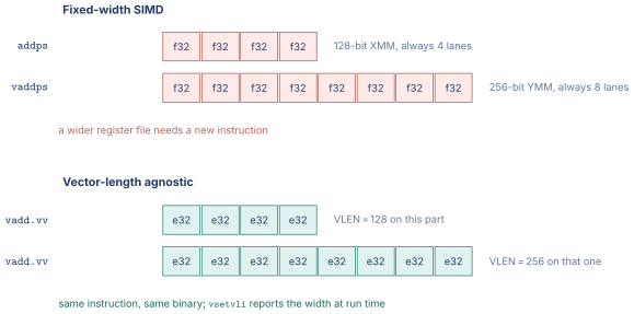
Figure 1 draws the difference: the same operation, once with the width baked into the mnemonic and once with the width left to the hardware.
The width treadmill, drawn
The difference between a fixed-width SIMD extension and a scalable vector one is easiest to see as a history rather than as a definition. Each time a fixed-width design widened its registers it had to add a fresh set of opcodes, and every program that wanted the new width had to be recompiled and often rewritten. Figure 2 puts the two histories on the same axis.
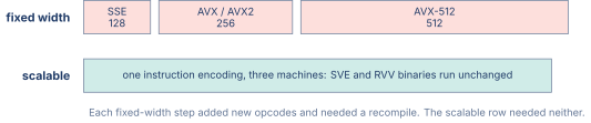
The cost of the top row is paid by software rather than by hardware. A library that wants to run well everywhere ships several compiled versions of its hot loops and selects among them at startup, a technique called function multiversioning. The source is written once, the loop bodies are written three times, and every new width adds a fourth. The bottom row replaces that with a single compiled loop whose trip count is read from the machine at run time.
What the bottom row gives up is the ability to name a width at compile time, and that turns out to matter for a narrow class of code. A kernel that lays out a fixed-size tile in registers, as a hand-tuned matrix multiply does, wants to know the register width while it is choosing the tile shape. Scalable code can query the width and branch, but it cannot bake the answer into a register allocation. This is why fixed-width intrinsics survive inside libraries even on machines that support scalable vectors.
02.The RISC-V V Extension
The RISC-V V extension [1] defines 32 vector registers (v0–v31), each VLEN bits wide. VLEN is an implementation parameter that the programmer does not hard-code. The minimum legal VLEN is 128 bits, but implementations may provide 256, 512, 1024, or more.
Setting the vector configuration
Every vector computation begins with a vsetvli (or vsetivli) instruction that establishes three parameters:
-
SEW (Selected Element Width): the width of each data element in bits. Legal values are 8, 16, 32, and 64.
-
LMUL (Length Multiplier): how many physical registers form one logical register. Legal values are 1, 2, 4, 8, , , and .
-
VL (Vector Length): the number of elements that subsequent vector instructions will process. The hardware computes VL as , where AVL is the application vector length (the number of elements remaining in the loop) and .
Setting vector configuration in RISC-V V assembly
| # a0 = number of elements remaining | |
| vsetvli t0, a0, e32, m1, ta, mu | |
| # t0 now holds VL (elements this iteration) | |
| # e32 -> SEW = 32 bits | |
| # m1 -> LMUL = 1 | |
| # ta -> tail agnostic | |
| # mu -> mask undisturbed |
A concrete example makes the arithmetic tangible. Suppose VLEN = 256 bits, SEW = 32, LMUL = 1. Then VLMAX = . If the application has 20 elements remaining, the first vsetvli sets VL = 8 and the loop processes elements 0 through 7. The second iteration sets VL = 8 again (elements 8 through 15). The third iteration has only 4 elements remaining, so VL = 4. Three iterations process all 20 elements.
With LMUL = 4, the same hardware provides VLMAX = . The 20-element array completes in a single iteration with VL = 20. The cost is that the 32 physical registers are grouped into 8 logical registers, reducing the register pressure budget.
Vector arithmetic and memory
Arithmetic instructions follow a uniform pattern: vadd.vv vd, vs2, vs1 adds corresponding elements of vs1 and vs2 into vd. The .vv suffix means both sources are vectors. The .vx suffix takes one scalar operand from a general-purpose register, and .vi takes a small immediate.
Memory operations use unit-stride, strided, and indexed forms:
Vector memory access patterns in RISC-V V
| # Unit-stride load: load VL consecutive 32-bit elements | |
| vle32.v v1, (a1) | |
| # Strided load: stride in a2 (bytes between elements) | |
| vlse32.v v2, (a1), a2 | |
| # Indexed (gather) load: offsets in v3 | |
| vluxei32.v v4, (a1), v3 |
The indexed load is the gather operation. Its counterpart, scatter, is vsuxei32.v. Gather and scatter allow vector code to operate on data structures with irregular access patterns, such as sparse matrices and hash tables, at the cost of lower throughput than unit-stride accesses.
Masking and tail handling
Any vector instruction can be predicated by setting the vm bit to 0 and designating v0 as the mask register. Element executes only if bit of v0 is 1. Masked-off elements follow the policy set by vsetvli: under “mask undisturbed” (mu) the destination element retains its old value, and under “mask agnostic” (ma) the hardware may write any value.
Tail elements are the elements beyond VL in the physical register. The tail policy is similarly configurable: “tail agnostic” (ta) allows the hardware to write ones or leave the elements unchanged, and “tail undisturbed” (tu) forces the hardware to preserve the old values. Tail agnostic is the common choice because it gives the microarchitecture more freedom and avoids false dependencies on the old register contents.
03.ARM NEON, SVE, and SVE2
ARM’s vector story spans two generations with fundamentally different design philosophies.
NEON: fixed-width SIMD
NEON [2] provides 32 registers (v0– v31), each 128 bits wide. Instructions operate on 2, 4, 8, or 16 elements depending on the element width (64, 32, 16, or 8 bits). The width is fixed at 128 bits, and the instruction encoding specifies the element arrangement.
A NEON ADD V0.4S, V1.4S, V2.4S adds four 32-bit integers. The .4S suffix is the “arrangement specifier” that tells the assembler the element count and width. Other arrangements include .2D (two 64-bit), .8H (eight 16-bit), and .16B (sixteen 8-bit).
NEON has no predication mechanism. If the loop trip count is not a multiple of the vector width, the programmer must handle the remaining elements with scalar code or masked stores, neither of which is elegant. This limitation motivated ARM to develop SVE.
SVE and SVE2: scalable vectors
The Scalable Vector Extension (SVE), introduced with the ARMv8.2-A architecture, brings the vector-length agnostic model to ARM. SVE registers (z0–z31) are between 128 and 2048 bits wide in multiples of 128. The actual width is an implementation choice. Software discovers it at run time.
SVE introduces 16 predicate registers (p0–p15), each with one bit per byte lane. Predication is first-class: every data-processing instruction takes a governing predicate. A whilelt instruction creates a predicate that is true for elements below the loop bound and false for the rest, replacing the scalar cleanup loop that NEON requires.
SVE loop adding two float arrays (conceptual)
| // x0 = array length, x1 = &a[0], x2 = &b[0], | |
| // x3 = &c[0] | |
| mov x4, #0 // index = 0 | |
| .loop: | |
| whilelt p0.s, x4, x0 // p0[i] = (i < len)? | |
| b.none .done // exit if no active lanes | |
| ld1w z0.s, p0/z, [x1, x4, lsl #2] | |
| ld1w z1.s, p0/z, [x2, x4, lsl #2] | |
| fadd z2.s, p0/m, z0.s, z1.s | |
| st1w z2.s, p0, [x3, x4, lsl #2] | |
| incw x4 // x4 += VL (in 32-bit words) | |
| b .loop | |
| .done: |
SVE2, ratified with ARMv9-A, extends SVE with additional integer, bitwise, and cryptographic operations. The register model and predication mechanism are unchanged.
04.Intel SSE, AVX, and AVX-512
Intel’s SIMD evolution spans four major generations, each doubling the register width.
SSE: the 128-bit era
Streaming SIMD Extensions (SSE), introduced with the Pentium III in 1999, added eight 128-bit XMM registers (xmm0– xmm7, extended to 16 with x86-64). Each register holds four 32-bit floats or two 64-bit doubles. SSE2 added integer SIMD operations on the same registers.
AVX and AVX2: the 256-bit era
Advanced Vector Extensions (AVX), introduced with Sandy Bridge in 2011, doubled the registers to 256 bits (ymm0– ymm15). AVX instructions use a three-operand VEX encoding that avoids the destructive two-operand pattern of SSE. AVX2 (2013, Haswell) extended 256-bit operations to integers.
The transition from SSE to AVX illustrates the fixed-width SIMD portability problem. An SSE addps xmm0, xmm1 and an AVX vaddps ymm0, ymm1, ymm2 are different instructions with different encodings. Compilers and libraries must provide separate code paths for each width, selected at run time via the CPUID instruction.
AVX-512: mask registers and 512-bit lanes
AVX-512, introduced with Knights Landing (2016) and Skylake-X (2017), expands registers to 512 bits (zmm0– zmm31) and adds eight dedicated mask registers (k0–k7).
The mask registers bring predication to x86 SIMD for the first time. An instruction like vaddps zmm0 {k1}, zmm1, zmm2 adds only the lanes where the corresponding bit of k1 is set. Masked-off lanes can be zeroed ({k1}{z}) or left unchanged (merge masking). This is conceptually similar to RISC-V V masking and ARM SVE predication, but AVX-512 remains a fixed-width ISA: the 512-bit width is encoded in the instruction.
AVX-512 also introduced gather and scatter instructions. VGATHERDPS zmm0 {k1}, [rax + zmm1*4] loads 16 floats from addresses computed as rax + zmm1[i]*4 for each lane where k1[i] is set. The corresponding scatter (VSCATTERDPS) writes elements to computed addresses.
The Intel APX and AVX10 direction
Intel’s AVX10 initiative converges the SSE/AVX/AVX-512 family into a single ISA extension with a configurable maximum vector width (AVX10/256 or AVX10/512). AVX10 guarantees that mask registers and the full instruction set are available at 256-bit width even on processors without 512-bit execution units. This partially addresses the portability gap between fixed-width SIMD generations, though it does not achieve the full vector-length agnosticism of RISC-V V or ARM SVE.
05.Comparison Across ISAs
The following table summarizes the vector and SIMD capabilities of the four architectures this book covers.
Table 1. Vector and SIMD ISA comparison
| Feature | RISC-V V | ARM SVE/SVE2 | ARM NEON | x86 AVX-512 |
|---|---|---|---|---|
| Width model | VLA | VLA | Fixed 128-bit | Fixed 512-bit |
| Min/Max width | 128 / impl. | 128 / 2048 | 128 / 128 | 512 / 512 |
| Data registers | 32 | 32 | 32 | 32 |
| Mask mechanism | v0 mask | pred. p0–p15 | none | k0–k7 |
| Tail policy | ta/tu config. | predicate-based | N/A | zeroing/merge |
| Gather/Scatter | yes | yes | no | yes |
| Element widths | 8/16/32/64 | 8/16/32/64 | 8/16/32/64 | 8/16/32/64 |
| LMUL grouping | yes (1–8) | no | no | no |
Two patterns emerge from this comparison. First, the vector-length agnostic ISAs (RISC-V V and ARM SVE) decouple software from hardware width. Second, predication (masking) is present in every modern vector ISA except NEON, reflecting the lesson that clean tail handling and conditional execution per lane are essential for writing efficient data-parallel code.
06.The Data-Parallel Execution Model
Regardless of whether the ISA is VLA or fixed-width SIMD, the execution model shares a common structure. A vector or SIMD instruction specifies:
-
An operation (add, multiply, shift, compare, etc.).
-
A set of source operands (two vector registers, or one vector and one scalar).
-
A destination register.
-
An optional mask that selects which lanes are active.
The hardware executes the operation on all active lanes. In a fixed-width SIMD machine, all lanes execute in a single cycle on parallel functional units. In a traditional vector machine (like the Cray-1 or a deeply pipelined RISC-V V implementation), elements are fed through a pipelined ALU one per cycle, and the instruction takes VL cycles to complete. From the programmer’s perspective, both models produce the same result. The microarchitectural difference affects throughput and latency but not correctness.
The data-parallel model maps directly to loops with no loop-carried dependencies. A loop body that reads a[i] and b[i], computes a[i] + b[i], and stores to c[i] has perfect DLP because every iteration is independent. Loops with dependencies between iterations (for example, a prefix sum where each element depends on the previous one) require additional techniques (segmented scans, reductions) that the vector ISA may or may not support directly.
07.Writing Portable Vector Code
The VLA programming model follows a canonical loop structure that works identically on RISC-V V and ARM SVE. The loop has four parts:
-
Configure. Set the element width and the number of active elements for this iteration (
vsetvlion RISC-V,whilelton ARM SVE). -
Load. Bring source data into vector registers using the active element count or predicate.
-
Compute. Perform the data-parallel operation on the active elements.
-
Store and advance. Write the results back to memory and increment the loop index by the number of elements processed.
RISC-V V: vector addition of 32-bit integer arrays
| # a0 = element count, a1 = &a, a2 = &b, a3 = &c | |
| .loop: | |
| vsetvli t0, a0, e32, m1, ta, ma | |
| vle32.v v0, (a1) | |
| vle32.v v1, (a2) | |
| vadd.vv v2, v0, v1 | |
| vse32.v v2, (a3) | |
| slli t1, t0, 2 # bytes = VL * 4 | |
| add a1, a1, t1 | |
| add a2, a2, t1 | |
| add a3, a3, t1 | |
| sub a0, a0, t0 | |
| bnez a0, .loop |
This loop has no hard-coded vector width. On a machine with VLEN = 128 it processes 4 elements per iteration. On a machine with VLEN = 1024 it processes 32 elements per iteration. The same binary works on both.
Fixed-width SIMD code (SSE, AVX, NEON) cannot achieve this portability at the assembly level. Compilers can auto-vectorize scalar C code for different SIMD widths, but the generated binary is width-specific. Libraries like Highway and SIMD Everywhere provide a source-level abstraction that maps to the native SIMD width at compile time, offering a practical middle ground.
08.Historical Context: From Cray to Modern Vectors
The vector processing idea predates the SIMD idea by two decades. CDC’s STAR-100 (1974) was a memory-to-memory vector machine that streamed its operands directly from memory and had no vector registers at all. Seymour Cray, who had left CDC in 1972 to found Cray Research, took the other approach in the Cray-1 (1976), which introduced vector registers and pipelined functional units that could sustain one floating-point result per clock cycle for long vectors. The Cray-1 had eight vector registers, each 64 elements of 64 bits. A single VADD instruction issued to the pipelined adder would produce 64 results over 64 cycles, amortizing the instruction fetch and decode cost over the entire vector.
The Cray approach dominated scientific computing through the 1980s and early 1990s. Japanese supercomputers (NEC SX series, Fujitsu VP) refined the model with longer vectors and deeper pipelines. The decline of dedicated vector supercomputers in the mid-1990s coincided with the rise of commodity microprocessors whose clock frequencies and cache hierarchies outpaced the vector machines for many workloads.
SIMD extensions emerged in the commodity world. Intel’s MMX (1997) packed eight 8-bit or four 16-bit integers into a 64-bit register repurposed from the x87 floating-point stack. SSE (1999) introduced dedicated 128-bit XMM registers. ARM’s NEON (2004) brought 128-bit SIMD to mobile processors. Each generation was a fixed-width extension that required new instructions and new code.
The VLA revival came from two directions simultaneously. ARM announced SVE in 2016, targeting the HPC market (Fujitsu’s A64FX processor in the Fugaku supercomputer was the first SVE implementation). RISC-V ratified the V extension in 2021, drawing heavily on the Cray vector model. Both designs recognized that the fixed-width SIMD proliferation (SSE, AVX, AVX2, AVX-512, each with its own intrinsics and code paths) was unsustainable for software ecosystems.
09.Reductions and Horizontal Operations
Not all data-parallel operations fit the lane-by-lane model. A reduction combines all elements of a vector into a single scalar result. Summing an array, finding the maximum element, and computing a dot product are reductions.
RISC-V V provides dedicated reduction instructions: vredsum.vs vd, vs2, vs1 adds all elements of vs2 to the scalar in element 0 of vs1 and writes the result to element 0 of vd. Other reductions include vredmax, vredmin, vredand, vredor, and vredxor.
ARM SVE uses predicated reductions: FADDV S0, P0, Z1.S adds all active elements of Z1.S (those where P0 is true) and writes the scalar sum to S0.
On Intel, horizontal operations (VHADDPS, VPHADDD) add adjacent pairs within a register. A full reduction of a 512-bit register typically requires multiple shuffle and add steps, making reductions more expensive on x86 than on architectures with dedicated reduction instructions.
A practical example illustrates the difference. To compute the dot product of two 16-element float vectors on AVX-512, the programmer first multiplies element-wise (VMULPS), producing a 16-element vector of products. Then the 16 products must be summed into a single scalar. The standard approach is a cascade of VSHUFPS (or VPERM2F128) and VADDPS operations that halve the number of active elements at each step: 16 to 8, 8 to 4, 4 to 2, 2 to 1. Four reduction steps are needed. On RISC-V V, the same dot product is a vfmul.vv followed by a single vfredusum.vs, which the hardware implements internally.
Why a reduction is not just another vector operation
Every operation so far has been lane-local. Lane three of the result depends on lane three of each input and on nothing else, which is what makes the hardware wide and simple. A reduction breaks that rule. Summing a vector into a scalar needs every lane to reach every other lane, and the hardware has to provide a path that lane-local instructions never needed. Figure 3 shows the two ways to arrange the arithmetic.
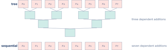
That last sentence is the part that constrains compilers. Floating-point addition is not associative, because each partial sum is rounded, so regrouping the additions can change the result. A compiler is therefore not permitted to convert a sequential floating-point accumulation into a tree unless the programmer says it may, which is what the fast-math family of flags and the #pragma omp simd reduction clause do. Integer reductions carry no such restriction and are vectorized freely.
This is the single most common reason a numeric loop refuses to vectorize. The loop looks parallel, every element is independent, and the only thing standing in the way is one accumulator variable whose additions the compiler is not allowed to reorder. The fix is to grant the permission explicitly rather than to restructure the loop, and the cost of granting it is that results may differ in the last few bits between one machine and another.
10.Vector Memory and Alignment
Vector loads and stores move large blocks of data between registers and memory. Three access patterns cover the vast majority of use cases.
Unit-stride accesses load or store consecutive elements starting at a base address. This is the most common pattern and the most efficient. Hardware can issue a single wide cache-line request when the address is aligned.
Strided accesses load every -th element, where (the stride) is specified in a register. Matrix column accesses in row-major storage and interleaved audio channels are typical strided patterns.
Indexed accesses (gather/scatter) use an index vector to compute per-element addresses. The hardware must issue separate memory requests for each unique cache line touched, making indexed accesses significantly slower than unit-stride or strided accesses.
Alignment requirements vary by ISA. RISC-V V permits naturally aligned and unaligned vector accesses (the hardware handles unaligned addresses transparently, though with a potential performance penalty). ARM SVE accesses are naturally aligned to the element size. Intel AVX-512 VMOVAPS requires 64-byte alignment, while VMOVUPS handles unaligned addresses.
Three access patterns and what they cost
A vector arithmetic instruction operating on eight lanes does eight times the work of its scalar equivalent. A vector memory instruction addressing eight lanes may or may not do eight times the work, and which of those is true depends entirely on where the eight elements sit. Figure 4 draws the three cases the ISAs give separate instructions for.

Unit stride is the case the hardware is built for. The elements share a cache line, the load is a single access, and the vector register fills at the width of the data path. Strided access divides the payoff by the stride until the stride exceeds a cache line, past which every element costs its own access. Gather is the general case, taking a vector of indices and performing what is architecturally one instruction and microarchitecturally up to one memory operation per lane.
The practical consequence is that data layout decides whether vectorization is worth anything. An array of structures stores the field a loop wants at a stride of the whole structure, which is the middle row of the figure. A structure of arrays stores the same field contiguously, which is the top row. Rewriting the layout is usually a larger win than any instruction selection, and no compiler will do it for you, because changing a data structure changes the meaning of every other piece of code that touches it.
11.Microarchitectural Considerations
The ISA defines what vector instructions do. The microarchitecture decides how fast they run. Two implementations of the same ISA can differ dramatically in vector throughput depending on the width of the execution units, the number of functional unit pipelines, and the memory subsystem bandwidth.
Execution unit width versus VLEN. An implementation with VLEN = 512 does not necessarily have a 512-bit-wide ALU. It might have a 128-bit ALU and process a 512-bit vector register in four beats (clock cycles). Each beat handles 128 bits, and the instruction takes four cycles to complete. From the programmer’s perspective, the instruction still processes VLMAX elements in one instruction. The difference is latency, not semantics.
Vector chaining. Vector chaining is a technique, pioneered on the Cray-1, where the result of one vector instruction is forwarded directly to the input of the next vector instruction on an element-by-element basis, without waiting for the entire vector to complete. If a vector multiply feeds a vector add, the first element produced by the multiplier can enter the adder one cycle later, while the multiplier is still working on subsequent elements. Chaining converts a sequential pair of vector instructions into a pipeline that overlaps their execution.
Not all microarchitectures implement chaining. Some read the full result from the vector register file before starting the next instruction. The ISA does not expose this choice. Software that depends on chaining for performance will run correctly on a non-chaining implementation, but the throughput may be lower.
Memory bandwidth. A single vector load can request many bytes from the cache in a single instruction. If VLEN = 512 and SEW = 32, a unit-stride load moves 64 bytes in one instruction. The cache port must be wide enough to supply those bytes in a reasonable number of cycles, or the load stalls the pipeline. In practice, many implementations have cache ports that are narrower than VLEN and service a vector load over multiple cycles. The balance between compute throughput and memory bandwidth determines whether a given workload is compute-bound or memory-bound.
12.Auto-Vectorization and Compiler Support
Most programmers do not write vector assembly by hand. Compilers perform auto-vectorization: they analyze scalar C or C++ loops, determine whether the loop body has sufficient data-level parallelism, and emit vector instructions automatically.
Auto-vectorization works best on simple loops with known trip counts, no loop-carried dependencies, and regular memory access patterns. The following C loop is a textbook candidate:
A loop suitable for auto-vectorization
| void add_arrays(float *c, const float *a, | |
| const float *b, int n) { | |
| for (int i = 0; i < n; i++) { | |
| c[i] = a[i] + b[i]; | |
| } | |
| } |
When compiled with gcc -O2 -march=rv64gcv (enabling the V extension), GCC emits a VLA vector loop that uses vsetvli, vle32.v, vfadd.vv, and vse32.v. The compiler handles the loop tail automatically.
Auto-vectorization fails when the compiler cannot prove that the iterations are independent. Pointer aliasing (where a, b, and c might overlap in memory) is the most common obstacle. The restrict keyword in C tells the compiler that pointers do not alias, enabling vectorization of loops that would otherwise be left scalar.
For loops that the compiler cannot auto-vectorize, programmers have three options. First, intrinsics: compiler-provided functions that map directly to vector instructions (e.g., __riscv_vadd_vv_i32m1 for RISC-V V, vaddq_s32 for NEON, _mm512_add_epi32 for AVX-512). Intrinsics give full control but are ISA-specific and verbose. Second, portable SIMD libraries like Highway, xsimd, or std::experimental::simd (the C++ Parallelism TS) that abstract over the underlying ISA. Third, hand-written assembly, which is reserved for the innermost kernels of performance-critical libraries.
13.Worked Examples
14.Exercises
References
- [1]Waterman, Andrew and Asanovi\'c (2024). “The RISC-V.”
- [2](2024). “ARM.”