RISC vs CISC and Other Classifications
September 8, 202651 min readintermediate
The previous chapter described the anatomy of an instruction set without passing judgment on which design choices are superior. This chapter adds history and classification. It traces the arc from the earliest…
The previous chapter described the anatomy of an instruction set without passing judgment on which design choices are superior. This chapter adds history and classification. It traces the arc from the earliest accumulator machines of the 1940s through the stack experiments of the 1960s, the general-purpose register revolution of the 1960s and 1970s, the RISC insurgency of the 1980s, and the CISC counterattack that followed. The conclusion is that the boundary between RISC and CISC has blurred almost to the point of irrelevance, and that a richer taxonomy is needed to describe modern instruction sets.
01.Operand Models: Where Do the Inputs Live?
Before asking how complex an instruction set should be, it helps to ask a more primitive question: where does an arithmetic instruction find its operands? Three answers have been tried in the history of computer design, and each one defines a class of machine.
The accumulator model
The earliest electronic computers had limited storage and even more limited wiring. The simplest way to build an arithmetic unit was to give it a single implicit register, the accumulator, and route every computation through that register. An “add memory” instruction fetches a value from a memory address and adds it to whatever is already in the accumulator. The result stays in the accumulator. A “store” instruction copies the accumulator to a memory address. The pattern for computing is:
Accumulator-style code for .
| LOAD A ; accumulator <- mem[A] | |
| ADD B ; accumulator <- accumulator + mem[B] | |
| STORE C ; mem[C] <- accumulator |
The EDSAC (1949), the IAS machine at Princeton (1952), and the early IBM 701 (1952) were all accumulator machines. The model is simple to implement because the ALU always reads one operand from the accumulator and one from memory, and always writes the result to the accumulator. The cost is traffic: every intermediate result that does not fit in the single accumulator must be stored to memory and loaded back later.
The stack model
The stack machine replaces the single accumulator with an implicit operand stack. A “push” instruction loads a value from memory and pushes it onto the stack. An “add” instruction pops the top two entries, adds them, and pushes the result. A “pop” instruction stores the top of the stack to memory. The same computation becomes:
Stack-machine code for .
| PUSH A ; push mem[A] onto stack | |
| PUSH B ; push mem[B] onto stack | |
| ADD ; pop two, push sum | |
| POP C ; pop result to mem[C] |
The Burroughs B5000 (1961) was the most celebrated stack machine. Its designers argued that the stack model maps naturally to the evaluation of arithmetic expressions, which compilers already convert to postfix (reverse Polish) notation internally. Java bytecode and the WebAssembly virtual machine both use a stack model at the specification level, though the hardware underneath is always a register machine. The JVM’s just-in-time compiler translates the stack-based bytecode into register-based machine code as part of its compilation pass, effectively undoing the stack representation before execution.
The appeal of the stack model is simplicity of encoding. Arithmetic instructions name no registers at all: the operands are implicit. This makes instructions short. The cost is that the stack’s strict last-in, first-out discipline makes it hard to keep frequently accessed values near the top. A computation that needs a value buried three entries deep must swap or duplicate stack entries, generating extra instructions. Compilers targeting stack machines tend to produce more instructions than compilers targeting register machines for the same computation.
The general-purpose register model
The general-purpose register (GPR) model gives the processor a file of named registers and lets arithmetic instructions specify their source and destination registers explicitly. The IBM System/360 (1964) was the landmark GPR design [1]. It provided 16 general-purpose 32-bit registers and a rich set of instructions that could name any register as source or destination. The CDC 6600 (1964), designed by Seymour Cray, had 24 operating registers organized into three specialized banks (8 address, 8 data, 8 index) and introduced many of the ideas that later became central to superscalar and out-of-order execution.
The GPR model won. Every commercially significant ISA since the mid-1970s has been a GPR machine. RISC-V has 32 registers. ARM A64 has 31. x86-64 has 16 (recently extended to 32 with APX). The reason is that a register file with entries can hold frequently used values simultaneously, reducing the number of loads and stores the program must execute. As Chapter 2 noted, memory access is far more expensive than a register read, and the gap has widened with every hardware generation.
The number of registers in the file is itself a design trade-off. More registers mean fewer spills to memory, but each additional register requires extra bits in every instruction to encode the register specifier. With 32 registers, each specifier is 5 bits. An R-type instruction that names three registers spends 15 of its 32 bits just on register specifiers. The IBM System/360 chose 16 registers (4-bit specifiers) in 1964, when every bit of encoding space was precious. The RISC designers of the 1980s chose 32, judging that the spill reduction justified the wider specifiers in a 32-bit instruction word. The trade-off has held stable since: no mainstream general-purpose ISA has gone above 32 architectural integer registers (though the x86-64 APX extension finally doubles from 16 to 32, decades after the RISC world settled on that count). The compiler-scheduled IA-64, covered later in this chapter, is the notable exception, defining 128 integer registers precisely because it moved instruction scheduling into software.
One expression, four operand models
The three models are easiest to tell apart by making all of them compute the same thing. Take the expression with all five variables in memory, and write it out for an accumulator machine, a stack machine, a two-address register machine and a three-address register machine.
The accumulator machine has one working register, so it can hold exactly one of the two products-in-progress at a time. It computes , and then it is stuck: the only place to put that value while it computes is memory. That store and the matching reload are not incidental. They are the direct consequence of having one register, and they are what the model costs.
The stack machine never names a register because it never has to. Each operator pops what it needs and pushes what it produced, so the expression tree is walked in postfix order and the code is a transcription of that walk. It is the shortest of the four in instruction count and the shortest in bytes, because an add that names nothing needs only an opcode.
The two-address register machine, which is what the 8086 and the System/360 look like at this level, gets closer but carries one recurring awkwardness: the destination is also a source, so any value that must survive the operation has to be copied first. The three-address machine has no such problem, and it is the only one of the four in which the code reads in the same shape as the expression.
Figure 1 puts the four side by side, with the instruction and byte counts under each.
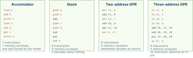
Two things in that figure are worth more than the instruction counts. The first is that instruction count and memory traffic move in opposite directions. The stack machine and the three-address machine tie on memory accesses at five, but the accumulator machine needs seven while executing the fewest instructions of any column except the two-address one. Counting instructions is a poor proxy for counting work, and the whole RISC argument turns on that distinction.
The second is that only the three-address column has no instruction that destroys one of its own inputs. That property is invisible in a listing this short and decisive in a long one, because a compiler allocating registers across a whole function is constantly asking whether a value is still live. On a two-address machine the answer is complicated by every arithmetic instruction; on a three-address machine it is not.
Why the stack model came back
The stack machine lost as a hardware design and then won somewhere else entirely, and the reason is instructive about what an ISA is for. The Java Virtual Machine is a stack machine. So is WebAssembly. So was the x87 floating-point unit that shipped in every x86 processor from 1980 until SSE2 displaced it, and that survives in the instruction set to this day.
The property that made the stack model bad in hardware is the same one that makes it good as an interchange format. Because operands are implicit, the encoding is compact and, more importantly, it is trivially verifiable. A validator can walk a WebAssembly function once, tracking only the height and types of the operand stack, and prove that no instruction ever pops from an empty stack or applies an integer operation to a float. That check is linear, needs no register allocation, and produces a definite answer before a single instruction runs. Doing the equivalent for a register machine means reasoning about which register holds what at every program point, which is a dataflow analysis rather than a scan.
So the stack model migrated to the layer where verification and density matter and where execution speed does not, because something else is going to translate it before it runs. Both the JVM and every production WebAssembly engine compile the stack code into register code before executing it. The stack machine is now a serialization format for expression trees, which is what it was always best at.
02.Memory Access Models: Load-Store versus Register-Memory
A second axis of classification asks which instructions can touch memory. Two answers dominate.
Load-store (RISC style)
In a load-store architecture, only dedicated load and store instructions access memory. Arithmetic instructions operate exclusively on registers. If a program wants to add a value from memory to a register, it must first load the value into a register, then add the two registers. RISC-V, ARM A64, and every other RISC ISA follow this model.
The load-store discipline makes the pipeline easier to design. The memory-access stage of the pipeline activates only for load and store instructions. Arithmetic instructions skip it entirely. This regularity simplifies hazard detection and forwarding logic, and it means that every arithmetic instruction has the same latency profile through the pipeline.
Register-memory (CISC style)
In a register-memory architecture, arithmetic instructions can have one operand in memory. x86-64 is the canonical example. The instruction ADD EAX, [RBX] reads a 32-bit value from the address in RBX, adds it to EAX, and writes the result to EAX. A single x86 instruction does what two RISC instructions (a load followed by an add) would do.
The register-memory model improves code density because fewer instructions are needed. The cost is pipeline irregularity. An instruction that accesses memory has a longer latency than one that does not. The decoder must determine whether the instruction touches memory before it can schedule it. In a modern out-of-order x86-64 processor, the decoder solves this problem by cracking the register-memory instruction into two micro-ops: one that performs the load and one that performs the add. The rest of the pipeline sees only uniform micro-ops, restoring the regularity that the ISA-level encoding obscured.
A subtler cost of register-memory instructions is that they complicate precise exception handling. If the memory access faults (because the address is unmapped), the processor must report the exception at the original instruction, not at the micro-op that performed the load. The retirement logic must track the correspondence between micro-ops and the ISA-level instructions they came from, adding bookkeeping that a load-store ISA avoids because each memory access is already its own instruction.
What register-memory costs the pipeline
The argument against register-memory instructions is usually stated as a matter of taste, and it is not. It is a matter of how many distinct things one instruction has to do before it can be called finished, and of what happens when one of those things fails partway through.
Consider add rax, [rbx + 8] on x86-64. Executing it means computing an address, reading memory at that address, adding the result to a register, and writing the register back. Those are four operations with three different kinds of latency: address arithmetic is a single cycle and always takes that long, the memory read is four cycles on an L1 hit and several hundred on a miss to DRAM, and the addition is again one cycle. A pipeline stage is a fixed amount of time. An instruction whose duration depends on whether a cache hit occurred cannot be assigned a fixed number of stages, so either the pipeline stalls for the worst case or the instruction has to be split.
Splitting it is what every high-performance x86 implementation does, and the split is exactly the load-store decomposition: one micro-op computes the address and performs the load, a second performs the addition. Figure 2 draws both paths through a simple five-stage pipeline so the difference in shape is visible.
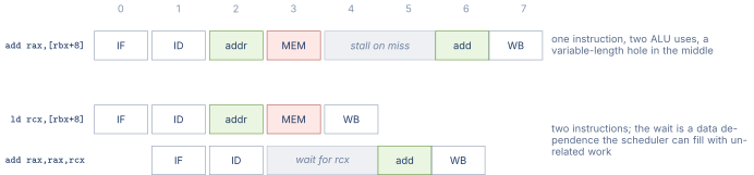
The stall is the same length in both timelines. What differs is whether anything else can happen during it. A hole inside a single instruction is not a scheduling opportunity, because the instruction is the unit the scheduler moves. Once the same work is two instructions, the gap between them is an ordinary read-after-write dependence, and every mechanism the machine has for hiding dependences applies to it.
There is a second cost, and it is the one that took longest to solve. A memory access can fault. If [rbx + 8] lies on an unmapped page, the instruction must be abandoned partway through, the operating system must map the page, and the instruction must then run again from the beginning. That requires that nothing observable has changed yet, which in turn requires that the register write be held back until the load is known to have succeeded. On a load-store machine the same requirement exists but is much easier to meet, because the faulting instruction does one thing and the arithmetic that follows it has not started. This is the precise exception problem from Chapter 13, and register-memory instructions make it harder in direct proportion to how much each instruction does.
03.Encoding Width: Fixed versus Variable
Chapter 13 introduced the distinction between fixed-width and variable-width encoding. The classification is worth revisiting here because it aligns closely with the RISC/CISC divide. Every RISC ISA that has achieved commercial success uses fixed-width 32-bit instructions (with optional 16-bit compressed forms). Every major CISC ISA uses variable-width encoding. The alignment is not coincidental.
A load-store ISA with a large register file needs three register specifiers (two sources and one destination) in most arithmetic instructions. Three 5-bit specifiers consume 15 of the 32 available bits. A 7-bit opcode, a 3-bit function selector, and a 7-bit function-extension field fill the rest. An instruction that needs a 12-bit immediate instead drops to two register specifiers, so 10 bits of specifiers, a 7-bit opcode, a 3-bit function selector, and the immediate again total 32. The 32-bit budget is tight but workable.
A register-memory ISA with complex addressing modes needs room for a base register, an index register, a scale factor, a displacement, and an immediate, in addition to the opcode and the destination register. Fitting all of these into a fixed 32-bit word is not practical. Variable-width encoding lets simple instructions be short and complex instructions be long, matching the encoding budget to the instruction’s actual needs.
The consequence for decoder design is substantial. A fixed-width decoder reads one aligned word and extracts fields at known bit positions. A variable-width decoder must scan the byte stream, identify prefix bytes, determine the opcode length, locate the operand specifiers, and compute the total instruction length before it can dispatch the instruction. Modern x86-64 processors invest a significant fraction of the front-end’s power budget in this pre-decode and length-detection logic.
The pre-decode problem is harder than it first appears. Consider a fetch window of 16 bytes. A fixed-width ISA with 4-byte instructions always contains exactly 4 instructions in that window, each starting at a 4-byte-aligned offset. A variable- width ISA does not know how many instructions the window contains until every instruction boundary has been found. The first instruction might be 2 bytes, the second might be 7 bytes, the third might be 4 bytes. Finding these boundaries requires sequential scanning from a known starting point. Modern x86-64 front ends use a pre-decode pipeline stage that marks instruction boundaries in the byte stream and caches the boundary information so that subsequent fetches of the same code region do not repeat the scan.
The real cost is finding the next instruction
The usual complaint about variable-width encoding is that decoding one instruction is complicated. That is true and it is not the expensive part. The expensive part is that you cannot decode the second instruction until you know where it starts, and you do not know where it starts until you have decoded the first.
On a fixed-width machine this problem does not exist. Fetch sixteen bytes, and if instructions are four bytes wide then there are four of them at offsets 0, 4, 8 and 12. Four decoders start work in the same cycle, in parallel, with no communication between them. Widening the machine from four-wide to eight-wide decode means adding four more decoders and nothing else.
On a variable-width machine the sixteen bytes might hold two instructions or sixteen. The second instruction begins wherever the first ends, so the decoders form a chain, and a chain of stages takes times as long as one. Figure 3 shows the two shapes.
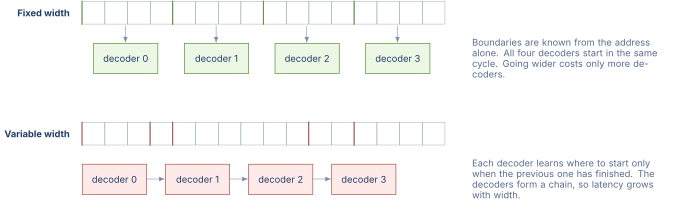
x86 implementations attack this from two directions. The first is to determine only the lengths in a separate early stage, before any instruction is fully decoded. Length determination is much simpler than decoding, since it needs to recognize prefixes, the ModRM and SIB bytes and the immediate size rather than work out what the instruction means. Even so, it is serial, and it is why x86 decode pipelines are longer than their fixed-width counterparts.
The second, and the one that actually solved the problem, is to avoid decoding the same bytes twice. The micro-op cache introduced with Sandy Bridge stores instructions in already-decoded form, keyed by address. Code inside a loop is decoded once on the first iteration and then supplied from the cache, with the legacy decoders powered down entirely. Since the overwhelming majority of dynamic instructions come from loops, most instructions on a modern x86 are never decoded from bytes at all after the first pass.
That is the honest resolution of the fixed-versus-variable debate, and it is not a victory for either side. Variable-width decode is genuinely harder, and the hardware that makes it acceptable is a cache that a fixed-width machine does not need to build. Apple’s M-series cores decode eight instructions per cycle with no micro-op cache at all, because on a fixed-width ISA eight-wide decode is eight decoders. The cost did not disappear. It moved into silicon area and design effort, where it is easier to pay and harder to see.
04.The Historical Arc
The ISA design space was explored in roughly chronological order. Accumulator machines came first because hardware was expensive and a single register was all the designers could afford. Stack machines came next as an attempt to match the hardware model to the compiler’s internal representation. GPR machines followed as register files became cheap enough to build at scale. The RISC philosophy then challenged the assumption that more complex instructions were always better. The history is worth knowing because the trade-offs that shaped each era still echo in modern design.
The accumulator era, 1940s–1950s
EDSAC (Cambridge, 1949), the IAS machine (Princeton, 1952), and the IBM 701 (1952) all organized computation around a single accumulator. The IBM 704 (1956) added three index registers for array addressing, a concession to the frequency with which scientific programs step through arrays. But the accumulator remained the central bottleneck. Every intermediate result had to pass through it, and programs spent a large fraction of their instructions moving data between the accumulator and memory.
A concrete measure of the cost: computing on an accumulator machine requires at least one store-and-reload cycle to park the intermediate sum before the multiply. On a GPR machine with three or more registers, the intermediate stays in a register and the store-and-reload is eliminated. For a computation with live intermediate values, an accumulator machine may need extra stores and loads. In floating-point-heavy scientific code of the 1950s, these extra memory accesses dominated execution time.
The stack interlude, 1960s
The Burroughs B5000 (1961) and its successors (B5500, B6700, B7700) were designed around a hardware-managed stack. The designers, led by Robert Barton, argued that the stack model was the natural match for Algol 60, the dominant high-level language of the era. Hewlett-Packard’s HP 3000 (1972) was another production stack machine. The approach produced elegant compilers but hit a performance ceiling as programs grew more complex and the strict stack discipline created too many redundant push-pop sequences.
The stack model’s fundamental limitation is that it turns every reuse of a buried value into extra instructions. If a computation needs the value three positions below the top of the stack, it must either duplicate or rotate stack entries to bring the value to the top. A register machine accesses any register in a single cycle regardless of when the value was written. For computations with many live temporaries (common in numerical code and in modern compiler intermediate representations), the register file’s random-access property is a decisive advantage.
The GPR revolution, 1960s–1970s
The IBM System/360 (1964) established the GPR model as the industry standard [1]. Its 16 general-purpose registers and its clean separation of integer and floating-point operations became the template for a generation of mainframes and minicomputers. The CDC 6600 (1964) pushed further, with multiple functional units that could execute different instructions simultaneously, anticipating superscalar design by two decades. The DEC PDP-11 (1970) brought the GPR model to minicomputers with 8 general-purpose 16-bit registers and a rich set of orthogonal addressing modes.
The CISC accumulation, 1970s
By the late 1970s, ISA designers had adopted the philosophy that complex instructions were desirable. The reasoning was straightforward: memory was slow and expensive, so packing more work into each instruction reduced the number of instruction fetches and improved code density. The DEC VAX (1977) was the culmination of this philosophy. It offered dozens of addressing modes, variable-length instructions from 1 to 54 bytes, and complex operations such as polynomial evaluation and packed- decimal arithmetic as single instructions. Intel’s 8086 (1978) was less extreme but still offered a variable-length encoding, segment-based addressing, and string-manipulation instructions that could move, compare, or scan entire arrays.
The RISC insurgency, 1980s
The RISC movement began with two academic projects in the early 1980s. At Berkeley, David Patterson and Carlo Séquin designed the RISC-I processor (1982), which had 32 registers, a fixed 32-bit instruction format, and only 31 instruction types. At Stanford, John Hennessy designed the MIPS processor (1984), with similar principles [2]. Both projects were motivated by an empirical observation: most of the complex instructions in CISC ISAs were rarely used by compilers, yet their presence in the ISA complicated every stage of the pipeline.
The key insight was that a simpler ISA could be clocked faster. If the hardware spent less time decoding complex instructions, it could spend more time executing simple ones at a higher rate. A RISC processor that executed one simple instruction per cycle could outperform a CISC processor that took three or four cycles to execute a complex instruction, even though the RISC program was longer. Patterson and Hennessy captured this argument in the processor performance equation:
The CISC approach reduced instruction count. The RISC approach reduced CPI (cycles per instruction) and clock cycle time. Whether the product was smaller for RISC or CISC depended on the magnitudes of each factor. The RISC proponents argued, correctly for the technology of the 1980s, that the CPI and cycle-time improvements more than compensated for the instruction-count increase.
The commercial fruits of the RISC movement were the MIPS R2000 (1985), the SPARC (1987, from Sun Microsystems), the IBM POWER (1990), the ARM (originally Acorn RISC Machine, 1985), the DEC Alpha (1992), and the HP PA-RISC (1986). Each followed the same core principles: fixed-width encoding, load-store memory model, large register file, and simple instructions designed to execute in a single pipeline stage.
The ARM story is worth a brief aside. Acorn Computers, a British company known for the BBC Micro, designed the original ARM processor in 1985 with a team of fewer than a dozen engineers. Sophie Wilson wrote much of the instruction set specification. Steve Furber led the hardware design. The first ARM chip had roughly 25,000 transistors, small enough that the entire design was done without any automated layout tools. The low transistor count and simple pipeline gave the ARM chip unusually low power consumption, a property that became the ARM franchise’s defining commercial advantage when mobile computing arrived a decade later. The original ARM was, in every sense, a product of the RISC philosophy: a simple, orthogonal instruction set designed for a small, fast pipeline.
The CISC counterattack, late 1980s–1990s
Intel’s response to the RISC challenge was not to abandon x86 but to build a RISC engine underneath it. The Intel 486 (1989) introduced a short pipeline and started executing simple x86 instructions in a single cycle. The Pentium Pro (1995) went further, translating each x86 instruction into one or more fixed-width micro-operations (micro-ops) at the front end and executing those micro-ops in an out-of-order, superscalar back end that was, internally, a RISC machine. AMD adopted the same strategy with the K5 (1996) and refined it through the Athlon and Zen families.
This approach worked. x86 processors matched and often exceeded the performance of RISC processors on general-purpose workloads by the late 1990s. The micro-op translation layer added area and power, but the x86 ecosystem’s enormous installed base of software justified the cost. The RISC ISAs lost their performance lead, and the market consolidated around x86 for desktops and servers and ARM for mobile devices.
05.Why the Distinction Blurred
By 2000, the sharpest claims of the RISC movement had been absorbed into mainstream practice. Every high-performance processor, regardless of its ISA classification, used deep pipelines, out-of-order execution, register renaming, and speculative branch prediction. The remaining differences between RISC and CISC ISAs were in the front-end cost of decoding and in code density, not in the execution engine’s architecture.
Several developments contributed to the blurring.
First, transistor budgets grew exponentially. The decoder complexity that made CISC impractical in 1985 became a small fraction of the total chip area by 2005. Modern x86-64 decoders consume a few percent of the core’s area.
Second, compilers improved. The RISC movement’s original argument partly rested on the claim that compilers rarely used complex CISC instructions. As compilers became more sophisticated, they began to exploit more of the ISA. At the same time, RISC ISAs added instructions that would have been considered “complex” by 1985 standards. ARM A64 has a fused multiply-add. RISC-V’s M extension has multiply and divide. The line between a “simple” and a “complex” instruction shifted.
Third, memory latency became the dominant bottleneck. Once the processor could execute instructions faster than memory could supply them, the execution model (RISC or CISC) mattered less than the cache hierarchy, the prefetcher, and the memory controller. Performance optimization shifted from instruction- level concerns to memory-level concerns.
Fourth, the market applied pressure toward convergence. Compilers, operating systems, and application binaries represent the ecosystem’s investment in an ISA. A RISC ISA that wanted to compete with x86 in the desktop market had to run x86 software somehow (through emulation, binary translation, or dual-boot), and an x86 processor that wanted to compete with RISC on performance had to adopt RISC microarchitectural techniques internally. The two sides met in the middle: RISC ISAs grew more complex (ARM added SIMD and crypto instructions), and CISC ISAs grew more RISC-like internally (micro-op translation, register renaming, deep out-of-order pipelines).
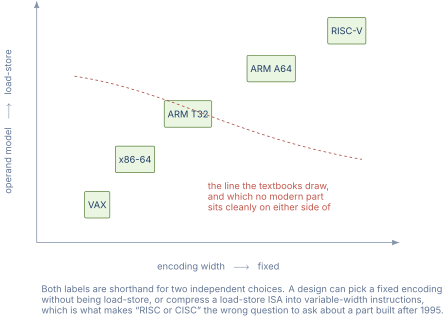
Figure 4 separates the two choices the labels compress.
What the RISC papers actually measured
The RISC argument is often repeated as a slogan about simplicity, which makes it sound like an aesthetic preference. It was not. It was an empirical claim, and knowing what was measured is what lets you judge how much of it still holds.
The measurement was of dynamic instruction mix: take real compiled programs, run them, and count how often each instruction is actually executed. The result that drove everything else was that a small number of simple instructions accounted for the overwhelming majority of executions, while the elaborate instructions the CISC ISAs had accumulated were almost never emitted by compilers at all. The VAX had an instruction that evaluated a polynomial and one that inserted an element into a doubly linked queue. Compilers emitted neither.
The inference was that those instructions were not free. Every addressing mode a compiler ignores still occupies encoding space, still appears in the decode logic, still has to be verified, and still constrains the microarchitecture, because the machine must remain able to execute it correctly if any program ever does. The proposal was to spend that silicon on things the common case uses: a larger register file, a deeper pipeline, a cache.
Two caveats belong with this, and the second is the one usually dropped.
The first is that the measurements were of the compilers of the late 1970s. An instruction a compiler does not emit may be unemittable in principle or may simply be beyond that compiler’s pattern matcher, and the two look identical in a dynamic trace. Some of the CISC instructions the RISC studies found unused were genuinely hard to target. Others were not targeted because nobody had written the pass.
The second is that the argument was about what to do with a fixed transistor budget, and that budget has grown by roughly five orders of magnitude since. A decoder that consumed a meaningful fraction of a 1980s die is a rounding error on a modern one. The RISC conclusion was correct and its premise has expired, which is why the performance gap the papers predicted never materialized in the market and why the argument had to move to power, where area still translates into something scarce.
Where the distinction still bites
Saying the labels have blurred is not the same as saying nothing follows from them. Three consequences of the original choices are still live, and none of them is about instruction count.
Decode power at the low end. Cracking, micro-op caches and length pre-decode all cost energy, and they cost it on every instruction fetched rather than on every instruction retired. On a server part running at 200 watts this is invisible. On a microcontroller with a 2-milliwatt budget it is the whole design. This is why the embedded market went to fixed-width load-store ISAs almost completely, and why the compressed extensions that recover code density there are still fixed-boundary schemes with two lengths rather than a free-form byte stream.
Code density where memory is the constraint. Instruction memory is not free in a part with 32 kilobytes of on-chip flash and no external memory at all. A 30 percent difference in code size is a 30 percent difference in what fits, and no amount of caching helps because there is no second level to cache from. Thumb-2 and RISC-V’s C extension exist entirely for this case.
The parts of the ISA that never blurred. Micro-op cracking translates one instruction into several. It cannot change how many architectural registers there are, and it cannot change the memory consistency model. Those two are visible to software, fixed at the ISA level, and unaffected by any implementation freedom. A machine with sixteen architectural registers spills more than one with thirty-two no matter how it is implemented internally, because the spilling is decided by the compiler against the architectural count. And a program correct under x86-64’s TSO can be broken by recompiling it for AArch64’s weaker model, which is a difference no decoder can absorb.
That last group is worth carrying forward. The RISC and CISC labels described encoding and operand decisions, which implementations have since made largely internal. They never described the register count or the memory model, which are exactly the parts of an instruction set that remain a genuine contract.
06.A Modern Taxonomy beyond RISC and CISC
If RISC versus CISC no longer captures the important distinctions, what does? Several orthogonal axes describe the design space more usefully.
Operand model
Accumulator, stack, or GPR, as discussed earlier in this chapter. The GPR model is universal in modern hardware, though the stack model persists in virtual machines (JVM, WebAssembly, Ethereum bytecode).
Memory access model
Load-store versus register-memory. ARM A64 and RISC-V are load-store. x86-64 is register-memory. The distinction matters for decoder and pipeline regularity.
Encoding strategy
Fixed-width, variable-width, or hybrid (fixed base with optional compressed forms, as in RISC-V with the C extension). The distinction matters for front-end power and decode bandwidth.
Execution model
In-order versus out-of-order. Scalar versus superscalar. The execution model is a microarchitectural choice, not an ISA choice, but some ISAs (notably VLIW and EPIC, discussed below) expose the execution model to software.
Parallelism model
SISD (single instruction, single data), SIMD (single instruction, multiple data), MIMD (multiple instruction, multiple data), and SIMT (single instruction, multiple threads, the GPU model). Flynn’s taxonomy from 1966 still provides a useful first-level classification. Modern processors combine several models: a single core is SISD for scalar code and SIMD when executing vector instructions, while the chip as a whole is MIMD with multiple independent cores.
VLIW and EPIC: the compiler-exposed approach
A very long instruction word (VLIW) processor bundles multiple operations into a single wide instruction word, and the compiler is responsible for filling each slot with an operation that can execute in parallel with the others. The Multiflow Trace and the Cydrome Cydra-5 of the late 1980s were early commercial VLIW machines. Intel’s Itanium (IA-64) was the most ambitious attempt. It used a variant called EPIC (Explicitly Parallel Instruction Computing) in which 128-bit “bundles” of three instructions carried a template field that told the hardware which operations could execute simultaneously.
The VLIW approach shifts scheduling complexity from the hardware to the compiler. The advantage is a simpler pipeline with no need for dynamic scheduling or register renaming. The disadvantage is that the compiler must know the pipeline latencies at compile time, which ties the binary to a specific microarchitecture. A VLIW binary compiled for a 4-wide machine runs poorly on a 6-wide machine because the compiler packed only 4 operations per bundle. This lack of binary portability across generations, combined with the difficulty of building a compiler that fills the wide bundles effectively, contributed to Itanium’s commercial failure.
VLIW survives in niche domains where the compiler can be tightly coupled to the hardware: digital signal processors (TI C6000 family), GPU shader compilers that target a known microarchitecture, and some network-processing engines. It has not succeeded as a general-purpose ISA strategy.
Why the same idea fails in a CPU and wins in a DSP
The split is sharp enough to be worth explaining, because it is not that DSP compilers are better. It is that a static schedule is a prediction about timing, and the two domains differ in whether that prediction can be made.
A VLIW compiler assigns each operation to a specific issue slot in a specific cycle. That assignment is correct only if every operation takes the latency the compiler assumed. A load that the compiler scheduled as four cycles and that misses to DRAM instead takes three hundred, and there is no mechanism in the ISA to express what should happen in between. The entire bundle stream stalls, including the operations that had nothing to do with the load, because the schedule is a fixed pattern and the machine cannot rearrange it.
Figure 5 shows what that costs against an out-of-order machine handling the same miss.
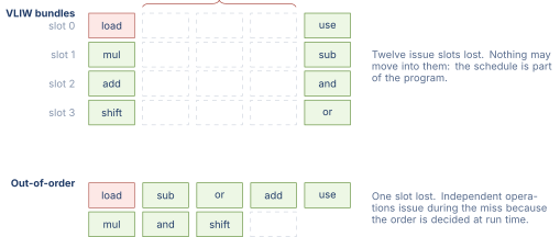
A digital signal processor runs the opposite kind of code. The working set is a filter’s coefficients and a block of samples, both of known size, and it is held in scratchpad memory that is addressed directly rather than in a cache. There are no misses to predict because there is no cache to miss in. Loop bounds are known at compile time, the branches are few and regular, and the same inner loop runs for the life of the product. Every assumption the static schedule rests on is true.
That is the actual condition for VLIW to work, and it is worth stating plainly because it is a statement about the workload rather than about the compiler: VLIW pays off exactly when instruction latencies are known at compile time. General-purpose code violates this constantly through the memory hierarchy. Signal-processing kernels do not violate it at all.
The same reasoning explains the third VLIW niche. A GPU shader compiler targets a known microarchitecture, ships with the driver, and recompiles the shader whenever the hardware changes, which removes the binary-compatibility problem that Itanium could never solve. Recompiling is free when the vendor controls the compiler and the program is delivered as source.
Data-flow and transport-triggered architectures
Two other models deserve brief mention. A data-flow architecture fires an instruction as soon as all of its input operands are available, with no program counter and no sequential instruction stream. The MIT Tagged Token Dataflow Machine (1980s) and the Manchester Dataflow Machine were research prototypes. Data-flow eliminates the need for explicit scheduling, but the overhead of tracking token availability made it impractical at scale. The concept survives in the data-flow graphs inside modern out-of-order engines, where the scheduler fires micro-ops based on operand readiness.
A transport-triggered architecture (TTA) programs the processor by specifying data movements between functional-unit ports rather than specifying operations. The operation is a side effect of writing data to a functional unit’s trigger port. TTA is an extreme form of compiler-exposed scheduling and shares VLIW’s binary-portability problems. It remains a research curiosity, though the TTA-based Processor Generator project at Tampere University has produced working FPGA implementations for DSP workloads.
Table 1. Summary of ISA classification axes with examples.
| Axis | Options | Examples |
|---|---|---|
| Operand model | Accumulator / Stack / GPR | EDSAC / B5000 / System/360 |
| Memory model | Load-store / Reg-memory / Mem-mem | RISC-V / x86-64 / VAX |
| Encoding | Fixed / Variable / Hybrid | ARM A64 / x86-64 / RISC-V+C |
| Parallelism | SISD / SIMD / MIMD / SIMT | Scalar / NEON / Multicore / GPU |
| Scheduling | Hardware (OoO) / Software (VLIW) | Zen 4 / Itanium |
07.Lessons for Modern ISA Design
The RISC-versus-CISC era left several enduring lessons that shaped every ISA designed after it.
Simplicity at the ISA level pays for itself in the microarchitecture. A regular instruction encoding makes the decoder smaller, faster, and lower power. The decoder runs on every instruction, so its cost multiplies by the instruction rate. A few percent of area saved in the decoder compounds across billions of instructions per second.
Backward compatibility outlasts performance arguments. Intel’s x86 survived the RISC challenge not because its encoding was better but because the installed software base was worth more than the decoder’s cost. ARM survived the transition from 32-bit A32 to 64-bit A64 because the A64 encoding was a clean redesign that kept the ecosystem continuity at the toolchain level even though the ISA encoding changed. RISC-V benefits from starting with no legacy at all.
The ISA is the specification, not the implementation. x86-64 is classified as CISC, but the execution engine inside a modern Intel or AMD core is as thoroughly pipelined, renamed, and out-of-order as any RISC core. ARM A64 is classified as RISC, but Cortex-X4 has a decode width of 10 and an issue width of 16, wider than most x86-64 cores. Classification labels describe the ISA’s encoding philosophy, not the chip’s actual architecture.
The performance equation is the arbiter. Whether an ISA design is good or bad depends on the product of instruction count, CPI, and clock cycle time, as the equation above states. No single factor dominates across all workloads and all technology nodes. The ISA designer’s job is to find the encoding that minimizes the product for the target workload and the target technology.
Energy efficiency has become the new performance. The RISC-versus-CISC debate of the 1980s centered on execution speed. Since the end of Dennard scaling around 2006, the conversation has shifted to energy per operation. A simpler decoder consumes less energy per instruction decoded. A fixed-width fetch consumes less energy than a variable-length pre-decode scan. ARM’s dominance in mobile and RISC-V’s growth in embedded are driven as much by energy arguments as by performance arguments. The decoder’s contribution to total core power is typically 5 to 15 percent in modern high-performance designs, and that fraction is higher in smaller, energy-constrained cores where the decoder is a larger share of the total area.
The number of ISAs is consolidating, not expanding. In the mid-1990s, at least eight commercially significant ISAs competed: x86, MIPS, SPARC, PA-RISC, Alpha, PowerPC, ARM, and 68k. By 2026, three dominate: x86-64, ARM A64, and the rising RISC-V. The consolidation is driven by ecosystem economics. Maintaining a compiler toolchain, an operating system port, a library ecosystem, and a developer community for an ISA costs billions of dollars over its lifetime. Only ISAs with a large enough installed base or a strong enough structural advantage (open licensing, in RISC-V’s case) can sustain that investment.
08.Worked Examples
09.Exercises
References
- [1]Amdahl, Gene M. and Blaauw, Gerrit A. and Brooks, Frederick P. (1964). “Architecture of the IBM.” IBM Journal of Research and Development, 8(2), pp. 87--101. doi:10.1147/rd.82.0087
- [2]Hennessy, John L. and Patterson, David A. (2019). “Computer Architecture: A Quantitative Approach.” Morgan Kaufmann.