Cache Organization, Policies, and Prefetching
September 8, 202644 min readadvanced
A read from main memory takes roughly 80 nanoseconds measured from the load instruction, once you include the core's queues, the interconnect, the memory controller's scheduler, and the trip back. Convert.
01.Part 1, why caches have to exist
1.1 The number that starts everything
One core at 3 GHz. One cycle is seconds, about 0.33 nanoseconds. Hold that.
A read from main memory takes roughly 80 nanoseconds measured from the load instruction, once you include the core's queues, the interconnect, the memory controller's scheduler, and the trip back. Convert.
Now say what that costs. A wide out-of-order core retires up to 6 instructions per cycle. Stall it for 240 cycles and you threw away the chance to retire about instructions. One memory access. Fourteen hundred instructions of lost opportunity.
That ratio is the memory wall, and it is a historical divergence rather than a law. Processor cycle time improved roughly 50 percent per year for two decades while DRAM latency improved about 7 percent per year. The gap compounded. In 1985 a memory access cost a handful of cycles and nobody cared.
1.2 Why you cannot just build one big fast memory
The obvious objection is to build main memory out of the fast stuff. Three reasons you cannot.
Cost per bit. An SRAM cell is six transistors. A DRAM cell is one transistor and one capacitor, in a process tuned for capacitors. Per unit area you get roughly an order of magnitude more DRAM bits, so 16 GB of SRAM is not slightly expensive, it is absurd.
Access time grows with size. A memory array is a grid with decoders on one side and sense amps on the other. Double the capacity and the wordlines and bitlines lengthen, raising their capacitance, slowing every access by exactly the reasoning in Digital Logic and Timing. Access time grows roughly like . A 32 KB array answers in a fraction of a nanosecond. A 32 MB array cannot, whatever it is built from, because the wires inside it are longer.
The speed of light. On-chip signals move at maybe m/s before RC delay and repeaters. In one 0.33 ns cycle that is about 5 centimetres, optimistically. A DRAM die centimetres away on a package cannot answer in a cycle no matter how good it is.
So a memory can be large, fast, or cheap, and you get two. The response is several memories at different points on that curve, arranged so the fast small one answers most of the time. That is the memory hierarchy, and a cache is any level that holds a subset of the level below and gets checked first.
1.3 Locality, and the workloads that have none
Caching only helps if the small fast memory usually has what you want, and there is no reason in principle for that to be true. A program touching uniformly random addresses across 16 GB would hit in a 32 KB cache about 0.0002 percent of the time.
Real programs are not random. Temporal locality means an address touched now is likely touched again soon, which is what makes it worth keeping a line. Loop counters, stack frames, and hot pointers produce it. Spatial locality means an address near one just touched is likely touched soon, which is what makes it worth fetching more than you asked for, and it is why caches move 64-byte lines rather than bytes. Arrays, instruction streams, and struct fields produce it.
Now the honest part, because a candidate who only knows the happy case is easy to catch. Workloads exist that defeat both at once. Pointer chasing through a large randomly-laid-out graph has no spatial locality, since each node sits at an unpredictable address, and no temporal locality, since a traversal visits each node once. Graph analytics, sparse matrix codes, and hash probing all look like this. A streaming scan over a buffer far larger than the cache has perfect spatial locality and zero temporal locality, so every line is fetched, used once, and evicted while the cache adds latency and burns power for nothing. Everything below either exploits locality harder or limits the damage when there is none.
02.Part 2, how a cache is actually built
2.1 The lookup problem
Given a 48-bit address, the cache must answer fast. Do I hold that data, and if so where.
The naive answer stores the full address beside every line and compares against all of them. That is a content-addressable memory from Arbiters FIFOs and CAMs, and above a few dozen entries it is unaffordable, because every entry needs a comparator and every lookup toggles all of them.
The trick is to use part of the address to choose where to look, so only a handful of comparators fire. The address gets carved into three fields. Understanding that carving is the single most-asked cache question in interviews.
2.2 The decomposition, worked completely
Take a 32 KB, 8-way set associative cache with 64-byte lines and 48-bit physical addresses.
A set is the group of ways an address is allowed to live in. Now carve. The offset picks a byte inside the line, needing bits. The index picks one of 64 sets, needing bits. The tag is what is left and must be stored so you can verify you found the right line.
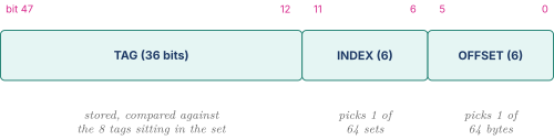
Read it bottom-up, since that is the order hardware uses it. The offset is ignored during lookup and only selects bytes at the end. The index drives a decoder that raises exactly one wordline. The tag is compared in parallel against the 8 tags in that row.
2.3 The lookup datapath
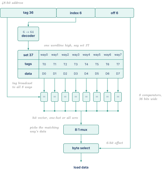
Two facts here follow you for the rest of your career. The tag compare and the data read happen in parallel, not in sequence, because sequencing them would nearly double hit latency. That means you read all 8 ways speculatively and discard 7, which burns power, and removing that waste is exactly what way prediction is for. And the whole chain, decoder plus array plus comparator plus mux plus byte select, must fit inside a 3 to 5 cycle L1 budget, which makes the tag path one of the most timing-critical structures on the die.
2.4 What the tags cost
Per line you store 36 tag bits, a valid bit, and a dirty bit. Per set you store replacement state, 7 bits for tree-PLRU on 8 ways as derived in 5.3.
A 32 KB cache really costs about 34.4 KB of SRAM. Now vary the line size and hold everything else fixed.
| Line size | Lines | Sets | Offset | Index | Tag | Overhead | Percent |
|---|---|---|---|---|---|---|---|
| 32 B | 1024 | 128 | 5 | 7 | 36 | 4976 B | 15.2 |
| 64 B | 512 | 64 | 6 | 6 | 36 | 2488 B | 7.6 |
| 128 B | 256 | 32 | 7 | 5 | 36 | 1244 B | 3.8 |
Halving the line size doubles the overhead, because you doubled the line count and each still needs a full tag. That is the first reason 8-byte lines are unthinkable. The second is that a bigger line exploits spatial locality for free. The third cuts the other way, since a bigger line fetches bytes you may not need, takes longer to transfer, and makes false sharing worse in a multiprocessor, which Cache Coherence Protocols covers. Sixty-four bytes is where those three forces balance.
Notice the tag stayed 36 bits in every row. Total size and associativity are fixed, so offset plus index is pinned at 12 bits, and moving a bit between them leaves the tag alone. Seeing that instantly is a good sign in an interview.
2.5 Direct mapped, set associative, fully associative
Associativity is how many places an address may live.
Direct mapped is one way. Lookup is as fast as it gets, one comparator, no way mux, and the data can even be forwarded before the tag compare finishes. The failure mode is brutal. Take a 32 KB direct-mapped cache with 64-byte lines, so 512 sets. Address 0x10000 indexes to . Address 0x18000 indexes to . Same set. A loop reading both misses on every access, at a 100 percent miss rate, in a cache that is 99.6 percent idle.
Fully associative is the other end. No conflict misses can exist by construction, the index field disappears, the tag grows to bits, and every lookup compares against every entry. For 512 entries that is 512 comparators per access. Unaffordable for a data cache, perfectly fine for a 32-entry TLB, which is why TLBs are fully associative and caches are not.
Set associative is what everyone builds.
| Direct mapped | 8-way | Fully associative | |
|---|---|---|---|
| Places per address | 1 | 8 | all 512 |
| Comparators per access | 1 | 8 | 512 |
| Tag width here | 39 bits | 36 bits | 42 bits |
| Conflict misses | severe | rare | none by definition |
| Replacement policy | none needed | yes | yes |
| Typical home | old L1s, some LLC slices | almost everything | TLBs, MSHR files |
Returns diminish fast. One way to two ways removes most conflict misses. Eight to sixteen usually buys very little and costs hit latency and power. The classic rule of thumb is that a direct-mapped cache of size performs about like a 2-way cache of size .
One constraint forces the L1 choice. A virtually indexed, physically tagged cache, covered in Virtual Memory and Memory Ordering, needs the index to fit entirely inside the page offset so the index bits are identical in the virtual and physical address. With 4 KB pages that is 12 bits, of which the offset already took 6, leaving 6 for the index. Then
Which is exactly why 32 KB 8-way was the standard x86 L1D for fifteen years. Apple uses 16 KB pages, relaxing the bound by four, which is one public reason Apple L1 caches are reported as much larger than the x86 norm.
03.Part 3, the three Cs plus one
3.1 The taxonomy and a conflict miss you can see
Every miss costs the same at the moment it happens. The taxonomy still matters because each category has a different fix, and picking the wrong fix wastes silicon.
Compulsory misses are first-ever touches. No cache of any size or associativity avoids them. Count them by simulating an infinite fully associative cache. Capacity misses happen because the working set exceeds the cache, so the line would have been evicted even with full associativity. Count them as misses in a fully associative cache of the real size, minus compulsory. Conflict misses happen because too many hot lines mapped to one set, so a line died while the cache had room elsewhere. Count them as real-cache misses minus fully-associative misses.
Make conflict concrete. A 4-way, 64-set, 64-byte-line cache, so 16 KB. Run this.
| for (i = 0; i < N; i++) | |
| sum += a[i] + b[i] + c[i] + d[i] + e[i]; |
Suppose all five arrays are 16 KB aligned, which allocators and static layout both love to do. Then is a multiple of 64, so a[0], b[0], c[0], d[0], and e[0] share index bits. Five lines, four ways. Under LRU every iteration evicts the line the next one wants. Miss rate goes to essentially 100 percent while the working set is 320 bytes in a 16 KB cache that sits 98 percent empty.
Three fixes work at three layers. Raise associativity to 8 so the five fit, which is hardware. Pad each array by one line so the index bits differ, which is what a compiler's array-padding pass does. Or hash the index by XORing some tag bits in, so addresses differing only in high bits land in different sets, which is what skewed and XOR-indexed last-level caches do.
3.2 The fourth C, and the fixes collected
In a multiprocessor there is a fourth category. Coherence misses happen because another core's write invalidated your copy. True sharing misses are unavoidable communication and represent real work. False sharing misses, where the other core wrote a different variable in the same 64-byte line, are pure waste and are fixable by padding. Cache Coherence Protocols works a full example.
| Miss type | Cause | Fix | Cost of the fix | What does not help |
|---|---|---|---|---|
| Compulsory | first ever touch | prefetching, larger lines | bandwidth, pollution | capacity, associativity |
| Capacity | working set > cache | bigger cache, software blocking | latency, area, power | more ways |
| Conflict | hot lines collide in a set | more ways, index hashing, padding | hit latency, power | a bigger cache may not help |
| Coherence, true | another core wrote it | nothing, it is real communication | anything | |
| Coherence, false | another core wrote the same line | pad and align to 64 B | footprint | ways or capacity |
The two rows that catch people are the last column entries in the middle. More associativity does nothing whatsoever for a capacity miss, and doubling the cache can shift which addresses collide without separating the specific ones that were colliding.
04.Part 4, write policies
4.1 Write-through versus write-back
A read miss has one behavior. A write has a choice, because there are now two copies and they can disagree.
Write-through sends every store to the next level as well. The level below is always current, eviction is trivial, coherence is simpler, and a parity error in the cache is recoverable because a clean copy exists below. The cost is traffic. Write-back updates only the cache and sets a dirty bit, writing the whole line down at eviction.
Quantify it, because "less traffic" is not an argument until it has numbers. A loop writes 4 bytes to each of 16 consecutive positions inside one 64-byte line. Under write-through that is 16 transactions to the next level, and if the interface moves 8 bytes minimum, 128 bytes of traffic for 64 bytes of updates. Under write-back it is zero traffic until eviction, then one 64-byte writeback. A counter incremented a million times generates one writeback under write-back and a million transactions under write-through.
Every level beyond a small L1 is write-back. Some L1 data caches are deliberately write-through into L2 for the reliability reason above, since a write-through L1 never holds the only copy and can recover from an error by simply invalidating. SRAM Arrays and ECC develops that, and it is a nice example of a policy chosen for reliability rather than speed.
4.2 Write-allocate versus no-write-allocate
The second and independent choice is what happens on a write miss. Write-allocate fetches the line first and then writes it, betting on reuse. No-write-allocate, or write-around, sends the store past the cache without allocating, betting against reuse.
Work the streaming case. A memset over 1 MB with a 32 KB cache. Under write-allocate every 64-byte line is first read from memory and then completely overwritten, so you read 1 MB you did not need and write 1 MB, for 2 MB of traffic, and you evicted the entire useful contents of the cache along the way. Under no-write-allocate you write 1 MB and disturb nothing. Half the traffic, no pollution.
Real designs capture most of that without switching policy by detecting full-line writes. If buffered stores cover all 64 bytes, there is no reason to fetch the old contents, since every byte is about to be overwritten. Software can signal the same thing with non-temporal store instructions.
The pairings are conventional, not mandatory. Write-back with write-allocate is standard because both bet on reuse. Write-through with no-write-allocate is standard because both bet against it.
4.3 Write buffers
Stores must not stall the pipeline, so they go into a write buffer that drains in the background, which is the store queue of Load Store and Memory Ordering seen from the cache side. Two behaviors matter. Write merging combines several stores to one line into a single transaction, which is what turned 16 stores into one writeback above. And a load must check the write buffer in parallel with the cache, because the newest value of an address may still be sitting there. Forgetting that check is a classic correctness bug and a classic interview trap.
05.Part 5, replacement policies
5.1 What perfect would look like
On a miss into a full set, something must go. The best possible answer is Belady's optimal, which evicts the line whose next use is furthest in the future. It is provably optimal and unimplementable, since it requires the future. It is still useful, because running it in a simulator gives the upper bound that tells you how much room a real policy has left.
Every real policy is a guess about the future built from the past. LRU guesses that the line unused longest will stay unused longest. Right often enough to dominate for fifty years, wrong often enough that a research literature exists to fix it.
5.2 True LRU and its bit cost
True LRU keeps an exact recency ranking of ways. Naming an arbitrary permutation of items takes
For 8 ways, and , so 16 bits per set. For 16 ways it is 45 bits.
The bit count is not the real problem. The real problem is that the state updates on every access including every hit, and the update is a reordering rather than a simple write, sitting on the critical path beside the tag compare. A common practical encoding uses an matrix where row column says "way was used more recently than way ", costing bits for 8 ways and updating one row and one column per access. More bits than the theoretical minimum, but the update is cheap combinational logic. Trading extra state for simpler update logic recurs everywhere in microarchitecture.
5.3 Tree-PLRU, drawn and traced
Tree-PLRU puts the ways at the leaves of a binary tree and keeps one direction bit per internal node. For ways there are internal nodes, so 7 bits for 8 ways instead of 16.
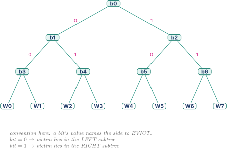
On an access to way , walk root to leaf and set each bit on the path to point at the other side. You just used this side, so the victim is over there. Three unconditional bit writes, no reordering. On an eviction, follow the bits down from the root. Three bit reads, and the leaf you land on is the victim.
Trace it. Fill an empty set by touching W0 through W7 in order.
| Access | Bits set on the path | State b0..b6 |
|---|---|---|
| start | 0 0 0 0 0 0 0 | |
| W0 | b0=1, b1=1, b3=1 | 1 1 0 1 0 0 0 |
| W1 | b0=1, b1=1, b3=0 | 1 1 0 0 0 0 0 |
| W2 | b0=1, b1=0, b4=1 | 1 0 0 0 1 0 0 |
| W3 | b0=1, b1=0, b4=0 | 1 0 0 0 0 0 0 |
| W4 | b0=0, b2=1, b5=1 | 0 0 1 0 0 1 0 |
| W5 | b0=0, b2=1, b5=0 | 0 0 1 0 0 0 0 |
| W6 | b0=0, b2=0, b6=1 | 0 0 0 0 0 0 1 |
| W7 | b0=0, b2=0, b6=0 | 0 0 0 0 0 0 0 |
Ask for a victim. Root b0 = 0, go left. b1 = 0, go left. b3 = 0, go left. Victim is W0, which is exactly true LRU. The approximation looks perfect.
Now break it, because that is the instructive part. Access W0 again, making it most recently used. That sets b0 = 1, b1 = 1, b3 = 1, giving 1 1 0 1 0 0 0. True recency is now W0, W7, W6, W5, W4, W3, W2, W1, so true LRU would evict W1. Ask the tree. b0 = 1, go right. b2 = 0, go left. b5 = 0, go left. Victim is W4, the fifth-most-recently-used line of eight.
That is the approximation error, and it happens because the tree remembers which half was touched recently, not the order inside each half. In exchange you got 7 bits instead of 16 and three unconditional writes instead of a permutation update. The miss-rate difference is usually well under a percentage point, which is why almost every real cache uses this.
5.4 RRIP and the problem LRU genuinely gets wrong
LRU has a failure that is not about approximation, it is about the underlying guess being wrong. When LRU brings a line in, it inserts it as most recently used, the most protected position in the set. That is a strong bet on reuse. For a streaming line that will never be touched again, the bet is exactly backwards. The new line evicts something useful, occupies the safest slot doing nothing, and does damage the whole way down. A scan longer than the associativity wipes the set.
RRIP, re-reference interval prediction, changes what the state means. Each line carries a 2-bit re-reference prediction value, an RRPV, predicting how far away its next touch is. RRPV 0 means very soon and is the most protected. RRPV 3 means distant if ever and is the eviction candidate. Three rules define SRRIP, the static version.
- On insertion, set RRPV = 2, meaning probably not soon but do not throw it out immediately. Note how different that is from LRU, which effectively inserts at maximum protection.
- On a hit, set RRPV = 0. The line proved itself, so promote it fully.
- On eviction, scan for any line with RRPV = 3 and evict the first found. If none, increment every RRPV in the set and scan again, repeating until a 3 appears.
Trace it on a 4-way set. The reused working set is A and B. The scan is S1 through S6.
| Access | Action | Set state after |
|---|---|---|
| A | miss, insert at 2 | A=2 |
| B | miss, insert at 2 | A=2 B=2 |
| A | hit, promote | A=0 B=2 |
| B | hit, promote | A=0 B=0 |
| S1 | miss, free way, insert at 2 | A=0 B=0 S1=2 |
| S2 | miss, free way, insert at 2 | A=0 B=0 S1=2 S2=2 |
| S3 | full, no 3, increment all, evict S1 | A=1 B=1 S3=2 S2=3 |
| S4 | S2 has 3, evict it | A=1 B=1 S3=2 S4=2 |
| S5 | no 3, increment all, evict S3 | A=2 B=2 S5=2 S4=3 |
| S6 | S4 has 3, evict it | A=2 B=2 S5=2 S6=2 |
| A | HIT | A=0 B=2 S5=2 S6=2 |
| B | HIT | A=0 B=0 S5=2 S6=2 |
A and B survived a six-line scan through a four-way set. Run the identical trace under LRU. The fill order is A, B, S1, S2, then S3 evicts A, S4 evicts B, S5 evicts S1, S6 evicts S2, and the final two accesses both miss. RRIP turned two misses into two hits.
Look at why, mechanically. The scan lines enter at 2 and are never hit, so they climb to 3 fast and become each other's victims. A and B entered at 2 but were hit, resetting them to 0, so they need three full increments before they are even candidates. Getting hit once buys a line a great deal of protection. Getting hit zero times buys it almost none. That is scan resistance, and it is the entire point.
5.5 DRRIP and set dueling
SRRIP still fails on a different pattern. A working set genuinely larger than the cache, scanned cyclically, still thrashes, because every line reaches 3 just before its next use. BRRIP, bimodal RRIP, inserts at RRPV 3 almost always and at 2 only about 1 time in 32. Inserting at 3 makes a new line an immediate candidate, so most of the resident set is preserved and a lucky few new lines survive, which keeps part of a too-large working set resident instead of cycling all of it.
Neither wins everywhere, so DRRIP picks between them at runtime by set dueling.
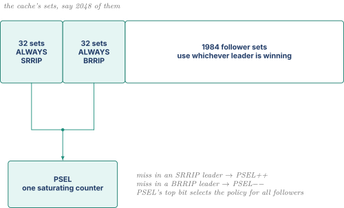
Dedicate a few leader sets to each policy permanently. Misses in one leader group increment a single counter, misses in the other decrement it, and the counter's top bit selects the policy for every follower set. Total cost is one 10-bit counter plus a comparison on index bits.
The elegance is that you are running a live A/B test on the actual workload, continuously, by sacrificing 64 sets out of 2048 to whichever policy is currently losing. The same trick gets reused for prefetcher aggressiveness, predictor component selection, and cache partitioning.
5.6 Random, FIFO, and an honest ranking
Random costs one LFSR shared by the whole cache and is surprisingly competitive at high associativity. It has one genuine advantage worth naming. It has no pathological input, since no adversary can construct an access pattern that makes it worst-case forever, which is not true of LRU. Some designs pick it specifically for that robustness. FIFO evicts the oldest-inserted line regardless of use, costs one pointer per set, and is generally worse than random because it discards information. It also exhibits Belady's anomaly, where a bigger cache can produce more misses on some traces, which stack algorithms like LRU provably cannot.
The ranking to carry is that LRU is not optimal, it is merely intuitive. It is a specific prediction that is right for reuse-heavy code and badly wrong for streaming and scanning code, and real workloads mix both. Every advanced policy is an attempt to detect which regime you are in, and set dueling is the cheapest detection anyone has found.
06.Part 6, the hierarchy
6.1 Levels, and what each is for
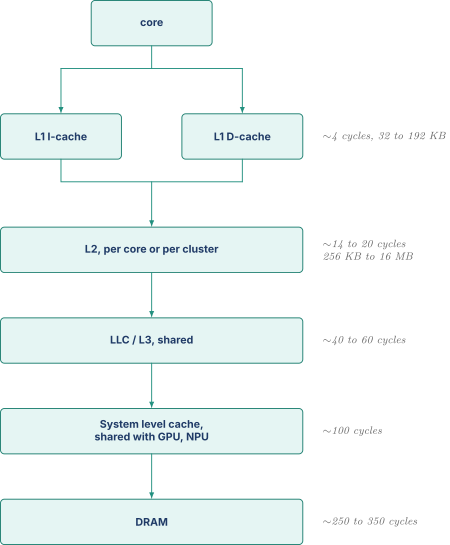
Each level exists because the one above is too small and the one below too slow. The instruction and data split at L1 is not about capacity, it is about ports. Fetch wants a wide read every cycle and load/store wants its own accesses, and one array serving both would need multi-ported SRAM, which costs far more than two single-ported arrays. Below L1 the streams merge because the bandwidth demand has dropped enough.
Apple adds a system level cache below the CPU hierarchy, shared with the GPU, neural engine, display, and image signal processor. That placement follows from a unified-memory SoC, where a buffer the CPU produces and the GPU consumes should ideally never reach DRAM. Reason about the mechanism rather than asserting internal numbers.
6.2 Inclusion, exclusion, and NINE
Does a line in L2 also have to be in L1. Three answers, and the coherence consequence is the reason anyone cares.
Inclusive guarantees everything inner is also outer. The payoff is large. An external snoop checks only the L2 tags, and if L2 does not have the line then by construction no L1 can, so the snoop is answered without touching the L1 at all. That preserves L1 tag bandwidth, which the core wants every cycle. The costs are duplicated capacity and back-invalidation, where an L2 eviction must reach up and kill the L1 copy, so the L2's replacement decisions can throw away a line the core is actively using. That pathology gets nasty when the inner-to-outer size ratio is small.
Exclusive puts a line in exactly one level, so effective capacity is the sum rather than the maximum. The costs are that coherence must check every level and that an L2 hit becomes a swap rather than a copy, since the L1 victim gets pushed down.
NINE, non-inclusive non-exclusive, guarantees nothing. No back-invalidates, no swaps, most of the capacity benefit. The price is that coherence needs help, which is where snoop filters come in, described in Cache Coherence Protocols. NINE plus a snoop filter is the common modern arrangement, and it is a clean example of adding a structure specifically to buy back a property a policy choice gave up.
6.3 AMAT, worked all the way down
These are local miss rates, the fraction of requests reaching that level which miss. The global miss rate of a level is the fraction of all core requests missing there, which is the product of local rates down to it. Confusing the two is a standard interview stumble.
Take , , , , , , , and work inside out.
Now perturb each input by a realistic amount, which is what turns arithmetic into judgement.
| Change | New AMAT | Delta |
|---|---|---|
| baseline | 6.80 | |
| 0.05 to 0.10 | 9.60 | +41 % |
| 4 to 5 | 7.80 | +15 % |
| 0.40 to 0.20 | 6.05 | -11 % |
| 40 to 30 | 6.65 | -2 % |
| 250 to 200 | 6.50 | -4 % |
The lesson is stark. One extra cycle of L1 latency costs more than shaving 10 cycles off L3 and 50 cycles off DRAM combined. That is why the L1 tag path gets fought over, why way prediction exists, and why L1 sizes moved so slowly. Everything near the core is leveraged by the sheer frequency of L1 accesses, and everything far from it is filtered by the levels above.
One caveat to raise if pushed. AMAT models a blocking machine where every miss costs its full latency serially. An out-of-order core overlaps misses, so the real penalty per miss is much smaller. AMAT is still the right first tool for comparing hierarchies, but it overstates miss cost on a machine with good memory level parallelism, which is Part 7. Performance teams quote MPKI, misses per thousand instructions, instead. If 30 percent of instructions are memory operations and the L1 miss rate is 5 percent, .
07.Part 7, non-blocking caches and MSHRs
7.1 The problem with stopping
A blocking cache handles one miss at a time. Miss, stall, wait 250 cycles, resume. In an out-of-order machine that is a catastrophe, because the entire point of Out of Order Execution is finding independent work while one instruction waits, and a cache that refuses a second request prevents the machine from finding that work even when it exists.
So caches became non-blocking. They keep serving hits while misses are outstanding, which is hit under miss, and accept further misses, which is miss under miss. That requires somewhere to record what is outstanding.
7.2 The MSHR file, primary and secondary misses
A miss status holding register tracks one outstanding line fill. The file is a small fully associative structure, typically 8 to 32 entries in an L1.
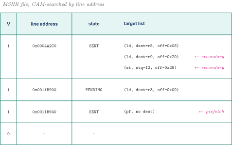
A primary miss is a miss to a line with no MSHR yet. It allocates an entry and sends a request downward. A secondary miss is a miss to a line that already has an MSHR. It sends no second request, it appends itself to that entry's target list and waits, and when the fill lands every target is satisfied at once.
That merging is worth a lot. A 64-byte line holds 16 four-byte integers, so an array traversal produces one primary miss and up to 15 secondary misses per line, and only the primary costs a memory transaction. Without merging you would issue 16 requests for the same line.
7.3 Little's law, and why MSHR count is a bandwidth ceiling
Little's law says that in any stable system the average number of items in flight equals arrival rate times time in system, . Apply it to memory. is the MSHR count, is memory latency in cycles, and is the sustainable miss rate per cycle, so .
Want one miss per cycle at . Then MSHRs, which nobody builds as a fully associative CAM in an L1. So run it the other way with 16 MSHRs.
That is a ceiling. It does not matter that DRAM can deliver 100 GB/s.
| MSHRs | Misses/cycle | Bytes/cycle | GB/s at 3 GHz |
|---|---|---|---|
| 4 | 0.016 | 1.0 | 3.1 |
| 8 | 0.032 | 2.0 | 6.1 |
| 16 | 0.064 | 4.1 | 12.3 |
| 32 | 0.128 | 8.2 | 24.6 |
| 64 | 0.256 | 16.4 | 49.2 |
State it plainly. Running out of MSHRs stalls the cache exactly as thoroughly as blocking would. The cache is non-blocking only up to outstanding misses and blocks beyond that. On memory-bound pointer-chasing code the limiter is usually neither DRAM bandwidth nor latency, it is that the machine cannot keep enough requests in flight, which is limited memory level parallelism. This is also a second reason prefetching helps, since prefetch requests occupy MSHRs and manufacture parallelism the demand stream could not generate.
Have a subtlety ready. MSHRs are not the only MLP limit. Load queue depth, reorder buffer size, the interconnect's outstanding-transaction limit, and the memory controller's queue depth all bound it, and the true limiter is the smallest. Asked to raise MLP, find which one binds before reflexively adding MSHRs.
7.4 Critical word first and early restart
A 64-byte line over a 16-byte interface takes 4 beats. The naive fill writes beats in address order then wakes the waiting load, so a load wanting byte 48 waited for all four beats. Critical word first reorders the transfer so the beat holding the requested word arrives first, wrapping around for the rest. Early restart wakes the waiting instruction as soon as its word lands rather than at the end of the line.
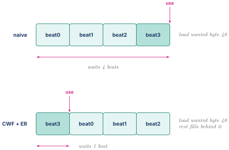
The saving is real but bounded at three beats of a transfer that already sat behind 250 cycles. It matters most when the transfer is a meaningful fraction of the total, which is far more true of L1 fills from L2 than of DRAM fills.
08.Part 8, prefetching
8.1 What it is for, and the four metrics
Everything so far is reactive. Prefetching is the one proactive mechanism. Predict the line, request it before the demand arrives, turn a miss into a hit.
Notice which C this attacks. Compulsory misses cannot be removed by capacity or associativity, because the data was never there. Prefetching is the only mechanism that removes them, and on streaming workloads compulsory misses are most of the misses. Prefetching is load-bearing, not marginal.
Judge any prefetcher on four numbers and be able to define each. Accuracy is the fraction of issued prefetches actually used before eviction. Coverage is the fraction of original demand misses eliminated. Timeliness is whether the line arrives in a useful window, since too late still stalls and too early gets evicted. Overhead is extra traffic, energy, cache pollution, and MSHR occupancy that demand misses now compete for.
8.2 Why accuracy and coverage trade
Take 1000 demand misses as a baseline.
| Design | Prefetches issued | Used | Accuracy | Coverage | Wasted traffic |
|---|---|---|---|---|---|
| conservative | 400 | 320 | 80 % | 32 % | 80 lines, 5 KB |
| moderate | 900 | 500 | 56 % | 50 % | 400 lines, 25 KB |
| aggressive | 3000 | 700 | 23 % | 70 % | 2300 lines, 147 KB |
Coverage rose from 32 to 70 percent while accuracy fell from 80 to 23. That is structural, not an artifact of these numbers. Covering more misses means issuing prefetches in situations you are less sure about, and less certainty means lower accuracy by definition. The only escape is a genuinely better predictor, which is why prefetcher work is fundamentally prediction work.
8.3 Timeliness, worked
A loop consumes one new line every 20 cycles. Memory latency is 250 cycles. The prefetcher runs lines ahead, the prefetch distance, buying cycles of lead time. For the line to have fully arrived,
At the lead time is 80 cycles, so the demand access still stalls cycles and recovers only 32 percent of the latency. Reporting "90 percent coverage" while every covered miss still stalled 170 cycles would be badly misleading, which is why coverage alone is not sufficient.
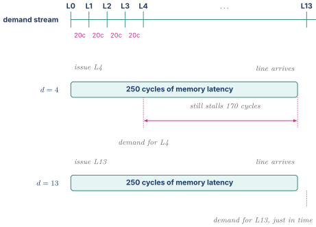
Push higher and a new failure appears. At there are 2560 bytes of speculative data in flight occupying cache and MSHRs, and if the loop exits early most of it was waste. Distance is itself an accuracy-versus-timeliness knob, and real prefetchers adapt it from observed usefulness.
8.4 The families
Next-line fetches line whenever line is touched. No table, no state, and remarkably effective on instruction fetch, where the program counter walks forward until a branch, and on linear data scans. Useless the instant the stride is not one line.
Stride learns a constant delta per instruction, held in a reference prediction table indexed by the load's PC.
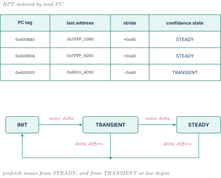
Work the example that shows why stride beats next-line. A 2D array of 32-bit integers with rows of 32 elements, so a row is 128 bytes, traversed column-wise.
| for (i = 0; i < 1000; i++) | |
| sum += a[i][j]; /* j fixed */ |
Consecutive accesses are 128 bytes apart, so every one lands on a different line, two lines apart. A next-line prefetcher fetches line , which is never the wanted line, giving zero accuracy and zero coverage while doubling traffic. A stride prefetcher sees deltas of , , , reaches STEADY in two or three accesses, and predicts perfectly afterwards. Same loop, opposite outcomes, and the difference is entirely which pattern the structure can represent.
Stream prefetchers work on address ranges rather than PCs. Detect that a region is being walked, allocate a stream buffer, run ahead by a configurable distance, and keep the fetched lines in that separate buffer rather than in the cache so a wrong guess evicts nothing. That separation of storage is the idea worth carrying.
Global history buffer prefetching decouples storage from indexing. Keep one circular FIFO of recent miss addresses plus an index table mapping a key, a PC or region or delta signature, into that FIFO with linked-list pointers. Because the history is stored once and indexed many ways, several algorithms share it and the history is always fresh rather than a stale per-entry snapshot.
Correlation and temporal prefetchers abandon regularity. Record that a miss to was historically followed by a miss to , then prefetch when misses again. A Markov prefetcher stores a few successors per address with confidence counters, and temporal streaming replays whole recorded sequences. This is the only family that touches pointer chasing, where addresses have no arithmetic relationship, only a historical one. The cost is enormous, and the table often lives in DRAM with its own cache.
| Family | Pattern caught | State cost | Typical home | Fails on |
|---|---|---|---|---|
| Next-line | stride of one line | none | L1I, L1D | anything else |
| Stride, RPT | constant delta per PC | small table | L1D, L2 | irregular, indirect |
| Stream | sequential region walk | few buffers | L2 | short streams, random |
| GHB | many, via one history | medium | L2 | needs a recurrence to exist |
| Correlation | arbitrary repeated sequences | very large | L2, LLC | first-time patterns |
An L1 prefetcher and an LLC prefetcher solve different problems with the same algorithms. An L1 prefetcher lives in 32 KB with 4-cycle latency, so a wrong guess evicts something the core is about to use and it is only hiding a 14-cycle L2 hit. It must be accurate, conservative, and short-distance. An LLC prefetcher displaces one line out of hundreds of thousands and is hiding a full 250-cycle DRAM latency, so pollution is cheap and the payoff for a right guess is 25 times larger. It can afford large tables and speculation. Saying that asymmetry out loud shows you are reasoning about a design point rather than reciting a taxonomy.
8.5 When prefetching makes things worse
This is the question that separates candidates, so carry mechanisms rather than a vague warning.
Bandwidth saturation, which is the big one and is a queueing argument. At utilization the average waiting time scales like . At that factor is 2, at it is 5, at it is 20. Take a workload already at and add an aggressive prefetcher contributing 60 percent more traffic. Utilization heads for , pins near 1, and the queue explodes. Every demand miss now waits behind a queue of mostly-useless speculative requests. The profile shows 70 percent prefetch coverage next to terrible performance, which is genuinely confusing the first time you see it.
Cache pollution. Useless lines occupy ways and evict live data, converting hits into misses, worst in small caches and at low accuracy. This interacts with replacement directly, which is why some designs insert prefetched lines at a less protected state than demand lines, for example RRPV 3 instead of 2, so a wrong prefetch dies fast.
MSHR occupancy. Section 7.3 showed MSHR count is a hard bandwidth ceiling. If 12 of 16 MSHRs hold speculative prefetches, the demand stream runs with 4 and its parallelism drops fourfold. Subtle and often missed.
Multicore interference. On a shared LLC and shared DRAM, one core's prefetcher steals bandwidth and capacity from another core that neither owns it nor can see it, which is a fairness problem as much as a performance one.
Power. A DRAM access costs on the order of hundreds of picojoules to a few nanojoules, against a few picojoules for a cache hit. A prefetcher running at 23 percent accuracy burns roughly four times the memory energy per useful line delivered. For a company shipping phones and laptops that argument carries as much weight as the performance one, and it is worth raising unprompted in an interview.
The answer to all of it is dynamic throttling. Count prefetch issues and prefetch hits, derive accuracy in hardware, and move the aggressiveness level up or down. Watch bandwidth utilization and back off when it is high. Use the set-dueling trick from 5.5 to A/B test aggressiveness live. Every modern prefetcher has a feedback loop, and the loop is often harder to get right than the predictor.
09.Part 10, check yourself
Answer out loud in full sentences, as though an interviewer asked. If you cannot, reread the section named.
- Convert an 80 ns memory access to cycles at 3 GHz and say how much work a 6-wide machine loses. Then give three reasons you cannot just build main memory out of SRAM. (1.1, 1.2)
- Define temporal and spatial locality, then name a workload with neither and say why. (1.3)
- Decompose a 32 KB 8-way 64-byte-line cache at 48-bit addresses, then compute the tag overhead as a percentage. (2.2, 2.4)
- What happens to overhead if you halve the line size, and why does the tag width not move. (2.4)
- Derive why 32 KB 8-way is such a common L1 size. (2.5)
- Give a loop that produces conflict misses in a 4-way cache and three fixes at three different layers. (3.1)
- Which of the three Cs does more associativity fix, and which does it do nothing for. (3.2)
- Work the traffic for 16 four-byte stores into one line under write-through and under write-back, then say why memset wants no-write-allocate. (4.1, 4.2)
- Derive true LRU's bit cost for 8 ways, draw tree-PLRU, count its bits, then give a case where the two choose different victims. (5.2, 5.3)
- Trace SRRIP on a 4-way set with a two-line working set and a six-line scan, and explain mechanically why the working set survives. (5.4)
- Explain set dueling. What does it cost and what does it buy. (5.5)
- Compare inclusive, exclusive, and NINE. Which needs a snoop filter and why. (6.2)
- Compute AMAT for the three-level example, then say whether you would rather have one cycle off L1 or fifty cycles off DRAM, with numbers. (6.3)
- Define primary and secondary misses, then use Little's law to get the per-core bandwidth ceiling with 16 MSHRs at 250-cycle latency. (7.2, 7.3)
- A loop consumes a line every 20 cycles at 250-cycle latency. What prefetch distance do you need, what breaks if you double it, and name four ways prefetching can make a program slower. (8.3, 8.5)
10.Part 11, related notes
- Cache Coherence Protocols for what happens when several caches hold the same line, including the fourth C and false sharing
- SRAM Arrays and ECC for what these arrays are physically made of, how they fail, and how they are protected
- Load Store and Memory Ordering for the store queue and load queue feeding the L1, and the ordering rules the cache must respect
- Virtual Memory and Memory Ordering for TLBs, VIPT, and where the physical address actually comes from
- Out of Order Execution for why non-blocking caches and memory level parallelism exist at all
- Arbiters FIFOs and CAMs for the CAM that an MSHR file and a fully associative cache are built from
- Interconnect and AMBA for the fabric a miss travels over once it leaves the cache
- Prefetching for the vault's deeper prefetcher treatment