Front End, Fetch, Decode, and Branch Prediction
September 8, 202651 min readadvanced
Out of Order Execution built a machine that holds 600 instructions in flight and issues 6 per cycle. Every structure in it, the rename tables, the reorder buffer, the issue queue, the physical register file…
01.Part 1, what the front end is actually for
1.1 The back end is a mouth that must be fed
Out of Order Execution built a machine that holds 600 instructions in flight and issues 6 per cycle. Every structure in it, the rename tables, the reorder buffer, the issue queue, the physical register file, exists to extract parallelism from a stream of instructions.
None of it produces instructions. Something upstream has to hand them over, six per cycle, forever, and they have to be the right ones.
That is the front end. Branch prediction unit, instruction cache, fetch, decode, and everything that keeps those four running at width. It is roughly a third of the core by area, it never idles, and it is where the two hardest problems in the machine sit next to each other.
1.2 Two failure modes, and they cost wildly different amounts
The front end fails in two structurally different ways, and separating them is the first thing to get straight.
Bandwidth failure. It delivers 3 instructions in a cycle when the back end wanted 6. Nothing is wrong, the instructions are correct, there just are not enough of them. The cost is exactly the shortfall, three instructions worth of issue slots that went unused this cycle.
Correctness failure. It delivers 6 instructions from the wrong path, because a branch was predicted incorrectly. Those instructions are fetched, decoded, renamed, dispatched, allocated ROB entries and physical registers, and some of them execute. Then all of it is thrown away.
The second is not a slightly worse version of the first. Work Part 1.3 and the ratio comes out at something like 50 to 1.
1.3 The arithmetic that sets the entire budget
From CPU Foundations Pipeline and Hazards, the CPI added by branch mispredictions is
where is the fraction of instructions that are branches, is prediction accuracy, and is the misprediction penalty in cycles.
Put real numbers on a wide, deep, modern machine. Take , meaning one instruction in five is a branch, which is typical of real integer code. Take cycles, which is roughly the distance from fetch to branch resolution in a machine of this class. And take the target IPC as 5, which means the base CPI is if nothing ever went wrong.
Now sweep accuracy.
| Accuracy | Total CPI | Actual IPC | Runtime vs the 99 percent case | |
|---|---|---|---|---|
| 99 percent | 0.232 | 4.31 | 1.00x | |
| 95 percent | 0.360 | 2.78 | 1.55x | |
| 90 percent | 0.520 | 1.92 | 2.24x |
Read the second row carefully, because it is the number this whole note exists to justify. Dropping accuracy from 99 percent to 95 percent, a change of four percentage points, costs 0.128 CPI. The entire base CPI of this machine is 0.2. So four points of accuracy added stall time equal to 64 percent of everything the machine does when it is working perfectly, and lengthened total runtime by 55 percent.
A second way to see it that is worth having in your head. At and 95 percent accuracy, the mispredict rate per instruction is , so the machine mispredicts once every 100 instructions and pays 16 cycles each time. At 99 percent accuracy it mispredicts once every 500 instructions.
Hold that 500 next to the 600-entry reorder buffer from Out of Order Execution section 4.6. Those two numbers being the same order of magnitude is not a coincidence. A window much larger than the distance between mispredictions is mostly full of instructions that will be discarded. The window size and the predictor accuracy are the same design decision seen from two ends.
1.4 Where the sixteen cycles physically go
The penalty is not a fixed constant handed down from a textbook. It is the distance between where a wrong-path fetch starts and where the mistake is discovered.
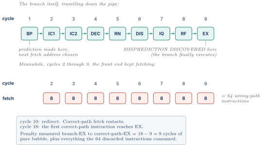
Two things fall out of that picture, and both get asked.
The penalty grows with pipeline depth, which is why deep pipelines and good predictors are coupled. A 20-stage machine has a bigger than a 12-stage machine, so it needs a better predictor to reach the same CPI. This is a large part of why chasing frequency by adding pipeline stages stopped working.
The penalty can exceed the pipeline depth. The formula assumes the branch executes as soon as it reaches the execution stage. If the branch depends on a load that missed to DRAM, it sits in the issue queue for 250 cycles before resolving, and the machine spends all of that time on a wrong path. This is why confidence matters, per 4.7, and it is the argument for predicting hard branches with an eye on how long they take to resolve.
And notice the resource cost buried in the diagram. Those 64 wrong-path instructions each took a ROB entry, a physical register, an issue queue slot, and real switching power. On a machine with a 600-entry window, a misprediction every 100 instructions means the window is chronically polluted.
02.Part 2, predicting direction, built from nothing
2.1 Static prediction, no memory at all
Start with the cheapest thing that could work. Guess the same way every time.
Always not taken is trivial, since the fetch unit simply keeps going to the next sequential address and needs no extra hardware at all. Roughly 60 percent of dynamic conditional branches are taken in real code, so this is right about 40 percent of the time. Worse than a coin flip.
Always taken inverts that and gets roughly 60 percent, but it needs the target, which means it needs the BTB from Part 5, so it is not actually free.
Backward taken, forward not taken, usually written BTFNT, uses one bit of information that is free. A branch whose target address is lower than its own address is almost certainly a loop back-edge, and loop back-edges are taken on every iteration but the last. A branch whose target is higher is probably an if skipping forward over a block, which is taken about half the time. So predict backward branches taken and forward branches not taken. This reaches roughly 65 percent and costs a single comparison on the sign of the displacement, which is already available in the instruction encoding.
Some ISAs also allow compiler hint bits in the branch encoding, set from profile-guided optimization. This works and is used, but it fixes the prediction at compile time, so it cannot adapt to a branch whose behavior differs between inputs.
Now feed 65 percent into the formula from 1.3 and see why none of this is enough.
That is added to a base CPI of 0.2, for a total of 1.32. The machine's IPC collapses from 5 to 0.76. A wide out-of-order core with a static predictor runs about six times slower than the same core with a good one. Every structure in Out of Order Execution is wasted silicon without dynamic prediction.
2.2 One bit of memory, and the loop that mispredicts twice
The obvious improvement. Remember what this branch did last time and guess it will do the same. That is a one-bit predictor, one bit of state per branch, holding the last outcome.
It should work well, because branches are extremely repetitive. Look at the case that matters most, a loop.
| for (i = 0; i < 10; i++) { | |
| body(); | |
| } |
The loop-closing branch is evaluated 10 times per pass. It is taken 9 times, jumping back for i equal to 0 through 8, and not taken once, falling out when i reaches 10. So the outcome stream for that one branch is
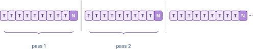
Trace the one-bit predictor across a pass, starting from state T because the previous pass ended taken. Actually, the previous pass ended not taken, which is the whole problem, so start from state N.
| Outcome # | Stored bit before | Predicts | Actual | Result | Stored bit after |
|---|---|---|---|---|---|
| 1 | N | N | T | MISPREDICT | T |
| 2 | T | T | T | correct | T |
| 3 to 9 | T | T | T | correct (7 more) | T |
| 10 | T | T | N | MISPREDICT | N |
Two mispredictions out of ten. Accuracy 80 percent on a branch that is 90 percent taken.
Now separate the two errors, because they are not the same kind of error.
The misprediction at outcome 10, the loop exit, is unavoidable for a predictor of this kind. The loop genuinely does end, and nothing in the last-outcome bit says when.
The misprediction at outcome 1, the loop re-entry, is pure self-inflicted damage. The branch is taken 90 percent of the time. The predictor knows this. But a single anomalous outcome, the exit, completely flipped its opinion, so it walked into the next pass predicting the wrong thing. One bit of state has no way to say "that was unusual, ignore it."
That is the problem. The predictor needs hysteresis, meaning resistance to changing its mind on a single piece of evidence.
2.3 Two bits, and why that is exactly enough
Give each branch a two-bit saturating counter instead of one bit. Four states, numbered 0 through 3.
| state 00 = strongly not taken (SN) | |
| state 01 = weakly not taken (WN) | |
| state 10 = weakly taken (WT) | |
| state 11 = strongly taken (ST) | |
| A taken outcome increments. A not-taken outcome decrements. | |
| Both SATURATE, meaning 11 stays at 11 on taken and 00 stays at 00 | |
| on not taken. | |
| THE PREDICTION IS THE HIGH BIT. Nothing else. |
The state diagram, which you should be able to draw from memory.
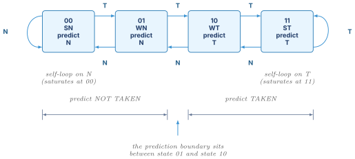
Now rerun the exact same loop. Start at state 11, ST, because the previous pass left it there.
| Outcome # | State before | Predicts | Actual | Result | State after |
|---|---|---|---|---|---|
| 1 | 11 ST | T | T | correct | 11 ST |
| 2 to 9 | 11 ST | T | T | correct (8 more) | 11 ST |
| 10 | 11 ST | T | N | MISPREDICT | 10 WT |
| next pass, 1 | 10 WT | T | T | correct | 11 ST |
| next pass, 2 | 11 ST | T | T | correct | 11 ST |
One misprediction out of ten. Accuracy 90 percent, up from 80.
Look at exactly where the improvement came from. At outcome 10 the loop exited and the counter went from 11 to 10. The prediction did not change, because the high bit is still 1. The counter recorded the surprise without acting on it. When the loop is entered again, the predictor is still saying taken, and it is right.
| One-bit | Two-bit | |
|---|---|---|
| Mispredicts per 10-iteration loop pass | 2 | 1 |
| Accuracy on that loop | 80 percent | 90 percent |
| Cost of one anomaly | flips the prediction | weakens it only |
| Storage per branch | 1 bit | 2 bits |
Why exactly two bits and not three or four? Because the gain runs out immediately. A three-bit counter has more hysteresis, which helps against a single anomaly, but it also takes three consecutive contrary outcomes to change its mind, so it adapts slowly when a branch genuinely changes behavior, which happens all the time in real programs when a phase changes. Measurements have consistently shown two bits to be the sweet spot, and two bits has been the standard building block for thirty years. Every predictor in Parts 3 and 4 is built out of these.
2.4 Where the counters live, and the first sign of trouble
You cannot afford a counter per branch address, because there are possible addresses. So build a table.
A pattern history table, or PHT, is an array of two-bit counters, indexed by some bits of the branch PC. AArch64 instructions are 4-byte aligned, so PC bits 1 and 0 are always zero and carry no information. Drop them and index with the bits just above.
Concretely, a 4096-entry PHT indexed by PC bits [13:2] costs bits, which is one kilobyte. That is nothing, and it is why even tiny embedded cores have one.
But now two different branches can land on the same entry.
| branch X at PC = 0x0000_1000 -> bits [13:2] = 0x400 | |
| branch Y at PC = 0x0000_5000 -> bits [13:2] = 0x400 <-- SAME ENTRY |
Those two PCs differ only in bit 14, which the index throws away. They now share one counter and update it with each other's outcomes. If X is almost always taken and Y is almost always not taken, they push the counter back and forth and both get predicted badly.
That is aliasing, and it is the enemy for the rest of Part 3.
03.Part 3, history, correlation, and the two-level idea
3.1 A branch that no per-branch counter can ever get right
Everything so far predicts a branch from its own past. Some branches are not predictable that way, and the example that shows it is worth working carefully because it motivates the entire modern field.
| if (x == 0) a = 1; // branch A | |
| if (y == 0) b = 1; // branch B | |
| if (x == 0 && y == 0) c = 1; // branch C |
A compiler turns each if into a conditional branch that jumps over the assignment when the condition is false. So the branch is taken exactly when the condition fails.
- Branch A is taken when .
- Branch B is taken when .
- Branch C is taken when NOT( AND ), which is when OR .
Tabulate all four cases.
| ? | ? | A taken? | B taken? | C taken? |
|---|---|---|---|---|
| yes | yes | N | N | N |
| yes | no | N | T | T |
| no | yes | T | N | T |
| no | no | T | T | T |
Stare at the last column. C is exactly the logical OR of A and B. Given the outcomes of the two immediately preceding branches, C is not a guess at all. It is a certainty.
Now ask what a per-branch two-bit counter for C can do. It sees only C's own outcome stream. If and are each zero half the time and independent, then C is taken in 3 of 4 cases, and its stream looks like a random sequence that is 75 percent taken. The counter saturates at strongly-taken and gets 75 percent. It cannot do better, ever, because the information it would need is not in the data it looks at.
This is the key idea and it is worth saying flatly. The limit is not the counter. The limit is the index. No amount of extra state per entry helps if you are indexing with the wrong thing.
3.2 The global history register
The fix is to make the outcomes of other branches part of the index.
A global history register, the GHR, is a shift register of the last branch outcomes across the whole program. On every branch, shift left by one and shift in a 1 for taken or a 0 for not taken.
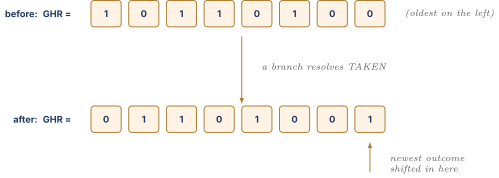
Now index the pattern history table with the GHR instead of the PC. For the example in 3.1, use a 2-bit GHR, which holds the outcomes of A and B at the moment C is predicted. That gives four table entries, and each one sees a constant outcome.
| GHR = (A, B) | Entry used | Outcome of C every single time | Counter converges to |
|---|---|---|---|
| N N | 00 | N | 00, strongly not taken |
| N T | 01 | T | 11, strongly taken |
| T N | 10 | T | 11, strongly taken |
| T T | 11 | T | 11, strongly taken |
After a brief warmup, 100 percent accuracy on C, with four counters totalling eight bits. The per-branch scheme was stuck at 75 percent with unlimited storage.
Two implementation details that separate people who have read about this from people who have thought about it.
The GHR must be updated speculatively. The prediction for the next branch is needed in the very next cycle, long before the current branch resolves. So the GHR is updated with the predicted outcome at predict time, not with the real outcome at execute time.
Which means the GHR must be checkpointed and restored. On a misprediction, the GHR contains a string of wrong-path predictions and is garbage. It has to be rolled back to the value it held at the mispredicted branch. That is exactly the checkpoint-and-restore machinery from Out of Order Execution section 6.3, applied to a second structure. By the end of this note there will be three structures needing it, the rename table, the GHR, and the return address stack.
3.3 The two-level taxonomy
Yeh and Patt organized this into a naming scheme that still gets used, and interviewers occasionally check that you recognize it. Every scheme has two levels. The first level records history. The second level maps a history pattern to a counter.
The name is three characters. The first says how history is kept, the middle A stands for adaptive, and the third says how the pattern tables are organized.
| Name | History (level 1) | Pattern table (level 2) | What it is good at |
|---|---|---|---|
| GAg | one Global history register | one global counter table | correlation between different branches, tiny storage |
| GAp | one Global history register | one counter table per branch address | correlation, without cross-branch interference, expensive |
| PAg | Per-address history, one register per branch | one global counter table | per-branch repeating patterns, like a fixed-trip-count loop |
| PAp | Per-address history | one table per address | most accurate in theory, absurd in storage |
Size the corners to see why only some are buildable. GAg with a 12-bit GHR needs counters, so 1 KB. PAp with 1024 tracked branches and 12 bits of local history each needs counters, which is 1 MB for a branch predictor. That is not happening.
The useful observation is that GAg and PAg are good at different things. GAg catches the correlated branch C from 3.1. PAg catches a loop that always runs exactly 4 times, since its local history TTTN TTTN repeats and the local pattern predicts the exit exactly. Neither dominates, which is the entire argument for hybrids in 3.6.
3.4 gshare, and what the XOR actually buys
GAg indexes by history alone, so every branch in the program with the same global history shares one counter. That is catastrophic aliasing.
The fix is to mix the PC back in. There are two ways.
gselect concatenates. Take bits of PC and bits of history and glue them together to form an -bit index. With a fixed budget of 12 index bits you might use 6 bits of PC and 6 bits of history.
gshare exclusive-ORs. Take 12 bits of PC and 12 bits of history and XOR them into a 12-bit index.
Why the XOR is better with the same table size is the actual question. With gselect and 12 index bits, you have thrown away 6 bits of PC and 6 bits of history before you started. Two branches whose PCs differ only in the discarded bits are permanently indistinguishable. With gshare and 12 index bits, all 12 bits of PC and all 12 bits of history contribute to the index. Nothing is discarded up front. You still get collisions, because the XOR maps input pairs onto entries, but the collisions are spread pseudo-randomly rather than being structurally guaranteed.
Work it concretely with 12-bit values.
| branch at PC bits [13:2] = 0x00A history GHR[11:0] = 0xB33 | |
| index = 0x00A XOR 0xB33 = 0xB39 | |
| SAME branch, different context: | |
| PC bits = 0x00A history = 0x000 | |
| index = 0x00A XOR 0x000 = 0x00A <-- different entry, good | |
| DIFFERENT branch, same history: | |
| PC bits = 0x1C4 history = 0xB33 | |
| index = 0x1C4 XOR 0xB33 = 0xAF7 <-- different entry, good | |
| an unlucky collision: | |
| PC bits = 0xB33 history = 0x00A | |
| index = 0xB33 XOR 0x00A = 0xB39 <-- collides with the first one |
So the same branch in two contexts gets two counters, two branches in the same context get two counters, and the residual collisions are the price. gshare is simple enough to describe in one sentence in an interview, which is exactly why it is asked about. XOR the global history with the branch PC and index a table of two-bit counters with the result.
3.5 Aliasing, measured and classified
Aliasing is not one phenomenon. Three cases, and only one of them hurts.
Destructive aliasing. Two branches share an entry and have opposite behavior. Each one pushes the counter toward its own answer, the counter thrashes in the middle, and both branches get predicted badly. This is the one that matters.
Neutral aliasing. Two branches share an entry and behave the same way. No harm at all, and arguably a small benefit, since the second branch arrives to find a counter already trained.
Constructive aliasing. Rare, where the shared training genuinely helps a branch that had not warmed up yet.
Estimate how much collision to expect. Take a 4096-entry table and 500 static branches active in a hot region. The number of distinct pairs is , and each pair collides with probability , so the expected number of colliding pairs is
Thirty colliding pairs out of 500 branches, and roughly half of those will be destructive because the branches disagree. That is a real and measurable accuracy loss, and it gets worse as the number of index bits used by history grows, because history multiplies the number of distinct (branch, context) entries competing for the same table.
Three responses exist. Make the table bigger, which works but costs linearly and eventually stops paying. Hash better, which is what gshare does relative to gselect. Tag the entries so an entry can say "that is not me," which is the idea that leads to TAGE in Part 4, and it is the only one of the three that actually solves the problem rather than diluting it.
There is also a targeted trick worth naming. A bi-mode or agree predictor splits the counter table into a mostly-taken half and a mostly-not-taken half and routes each branch to the half matching its bias. Branches sharing an entry then almost certainly agree, so aliasing becomes neutral instead of destructive without any increase in total storage.
3.6 Tournament predictors and the chooser
Section 3.3 ended with the observation that global-history and local-history schemes are good at different branches. The obvious response is to build both and pick.
A tournament or hybrid predictor runs two or more predictors in parallel and adds a chooser, itself a table of two-bit saturating counters, that learns which component to trust for each branch or each history context.
The Alpha 21264 is the canonical example and its sizes are worth knowing because they show the proportions.
| Component | Structure | Storage |
|---|---|---|
| Local predictor | 1024 entries of 10-bit local history, feeding 1024 three-bit counters | bits |
| Global predictor | 12-bit GHR indexing 4096 two-bit counters | 8192 bits |
| Chooser | 4096 two-bit counters, indexed by the GHR | 8192 bits |
The crucial detail about the chooser, and it is a good question to be asked. The chooser updates only when the two component predictors disagree. If both were right, or both were wrong, nothing was learned about which is better, and updating would inject noise. Only a disagreement is evidence, and then the counter moves toward whichever one was correct.
Hybrids were the state of the art for a generation, and the idea of combining specialists with a learned arbiter never went away. It reappears in Part 4 as the statistical corrector.
04.Part 4, the predictors that actually ship
4.1 Why any single history length is wrong
Every scheme in Part 3 picks one history length and lives with it. That choice is a genuine dilemma.
Short history, say 4 bits. Only 16 distinct patterns per branch, so each pattern is seen often and the counters train in a handful of executions. Warms up almost instantly. But it cannot possibly capture a correlation with a branch that executed 20 branches ago, because that outcome fell off the end of the register.
Long history, say 30 bits. Captures deep correlation. But there are , over a billion, distinct patterns. A branch executed 10,000 times in the whole program will essentially never see the same 30-bit history twice. Every lookup is a cold entry. The predictor never trains on anything.
Quantify the crossover. With an 8-bit history a branch sees at most 256 distinct contexts, so 10,000 executions give roughly 39 training samples per context, which is plenty. With a 20-bit history it sees up to a million contexts and 10,000 executions give 0.01 samples per context, which is nothing.
So short histories work for most branches, long histories are essential for a few, and a fixed choice is wrong for both populations. That is the problem TAGE solves, and its solution is elegant enough to be worth understanding properly.
4.2 TAGE, and why the history lengths are geometric
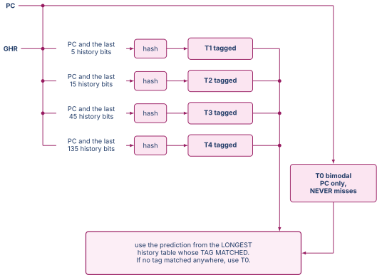
TAGE stands for TAgged GEometric history length predictor. It is several tables at once.
T0 is a plain bimodal predictor, PC-indexed two-bit counters, untagged. It always produces an answer, and it is the fallback.
T1 through Tn are tagged tables. Table is indexed by a hash of the PC together with the most recent bits of global history, where the history lengths grow geometrically.
With and , the four tagged tables use histories of length 5, 15, 45, and 135.
Now the question an interviewer will ask. Why geometric rather than evenly spaced?
Count what linear spacing would cost. To cover 5 through 135 in steps of 5 needs 27 tables. Geometric spacing with covers the identical range with 4.
That is the mechanical answer. The deeper answer is that the useful information in history grows sub-linearly with length. Going from 5 bits to 10 bits of context adds a lot. Going from 100 bits to 105 bits adds almost nothing, because a branch that needs 100 bits of context is already in a nearly-unique situation. So you want the sample points packed densely where the derivative is steep and spread out where it is flat, which is exactly what a geometric series does.
4.3 Why the tags are the whole trick
Take the tags away and TAGE collapses into a bank of gshare predictors, which is worse than one good gshare.
Here is why. An entry in the 135-bit-history table is indexed by a hash of a very specific situation. If the current branch has never been in that situation before, the entry it lands on holds a counter trained by some completely unrelated branch in a completely unrelated context. Without a tag, the predictor has no way to know this, and it will confidently report that stale counter's value. Long-history tables would be pure noise generators.
Add a tag, say 10 bits from a different hash of the PC and history, stored alongside the counter. Now the table only answers when the tag matches, which means "I have genuinely seen this exact branch in this exact history context before, and this counter is about it." Otherwise the table stays silent and the machine falls back on a shorter table or on T0.
That converts an unusable structure into the most powerful one in the predictor. The tag is what lets a table admit it does not know. Say it that way in an interview and it lands.
The prediction rule is then one line. Use the longest-history table that hits. Short-history tables cover the many easy branches, long-history tables answer only for the few branches that genuinely need deep context, and nothing in between wastes capacity.
4.4 Allocation, and the useful counter
Two more pieces make it work, and knowing them signals real reading rather than a summary.
Allocation on misprediction. When the providing component gets a branch wrong, TAGE allocates a new entry in a table with a longer history than the provider, not in the longest table. Usually just one new entry per misprediction. So a branch climbs the tables gradually, using the shortest history that suffices, and only branches that keep being wrong get promoted to deep history. That is what keeps the expensive long-history capacity reserved for the branches that need it.
The useful counter. Each tagged entry carries a small counter, usually 1 or 2 bits, called . It is incremented when that entry made a correct prediction that differed from what the next-shorter alternative would have said, meaning the entry earned its place. Allocation prefers to steal entries with . Without this, the tables fill up with entries that happen to agree with T0 and provide no value, and there is nothing left to allocate. The counters are also periodically reset in a graceful way, so an entry that was useful long ago in a dead program phase eventually becomes reclaimable.
4.5 Perceptron predictors, and the honest tradeoff
A completely different route to long histories.
Concretely first. Give a branch a set of small signed integer weights, through , say 8 bits each. Map the global history bits to , with taken becoming and not taken becoming . Compute
and predict taken if . The term is a bias with no history bit attached, capturing the branch's overall tendency.
Work an example with 4 history bits.
| weights w0 = +2 w1 = +7 w2 = -3 w3 = +1 w4 = 0 | |
| history (bias) T N T T | |
| as +/-1 +1 -1 +1 +1 | |
| y = 2 + (7)(+1) + (-3)(-1) + (1)(+1) + (0)(+1) | |
| = 2 + 7 + 3 + 1 + 0 | |
| = 13 -> positive -> PREDICT TAKEN |
Read the weights as opinions. says "when the branch one back was taken, this branch is strongly taken." says "when the branch two back was taken, this one leans not taken." says "the branch four back tells me nothing." That interpretability is not decoration, it is the mechanism by which a perceptron ignores irrelevant history bits, which a table cannot do, since a table treats every bit of the index as equally load-bearing.
Training. If the prediction was wrong, or if was below a threshold meaning the prediction was weak, then for each update where is if the branch was actually taken and otherwise, and update .
Continue the example, supposing the branch was actually not taken, so .
| Weight | Before | After | ||
|---|---|---|---|---|
| (bias) | +2 | n/a | +1 | |
| +7 | +1 | +6 | ||
| +1 | +1 | 0 | ||
| 0 | +1 |
Every weight moved slightly toward explaining the outcome. Nothing jumped.
The reason anyone uses this. Storage grows linearly with history length, not exponentially. A 60-bit history needs 61 weights of 8 bits, so 488 bits per perceptron. A table-based scheme with 60-bit history needs counters. That is the entire argument, and it is decisive.
The honest limitation, which is the good interview answer. A perceptron computes a weighted sum and thresholds it, so it can only learn functions that are linearly separable in the history bits. If a branch's outcome is the XOR of two earlier branch outcomes, no assignment of weights represents it, and the perceptron is stuck at 50 percent. A table-based scheme gets XOR for free, because each of the four history patterns has its own counter and each counter learns a constant. So tables and perceptrons fail on different branches, which is precisely why the winning designs use both.
The second limitation is timing. Computing a dot product of 60 terms is an adder tree several levels deep, and that does not fit in one cycle at a high clock. Real implementations pipeline it or compute it ahead of time, starting the sum several cycles before the prediction is needed, which is only possible because the older history bits are already known.
4.6 TAGE-SC-L, and the loop predictor that closes 2.3
What actually wins the Championship Branch Prediction competitions, and what production designs resemble, is TAGE-SC-L, three components combined.
TAGE is the main engine, per 4.2 through 4.4.
SC, the statistical corrector, is a perceptron-style component that watches TAGE and learns the situations in which TAGE is systematically wrong, then flips the prediction. This is exactly the hybrid idea from 3.6 with a smarter arbiter, and it is where the linear-separability strength of perceptrons complements the pattern-table strength of TAGE.
L, the loop predictor, detects branches that form loops with a constant trip count, counts iterations, and predicts the exit exactly.
That last component is worth pausing on, because it closes the loop opened in section 2.3. The two-bit counter still mispredicted once per loop pass, on the exit, and we called that unavoidable. It was unavoidable for that predictor. A loop predictor that has observed the loop run exactly 10 times on several passes simply counts to 10 and predicts not-taken on the tenth, taking that residual misprediction to zero. On a tight loop executed thousands of times, that is a real win, and it is the reason a specialized component earns its area.
4.7 Confidence, which is what the rest of the machine wants
A predictor can report more than taken or not taken. It can report how sure it is, derived from whether the providing counter is saturated or weak, how long the providing table's history is, and how high that entry's useful counter has climbed.
Three consumers use that.
Selective checkpointing, per Out of Order Execution section 6.3, spends its limited rename-map checkpoints on low-confidence branches, since those are the ones likely to need fast recovery.
Section 1.4 noted that a branch waiting on a DRAM miss spends hundreds of cycles on a possibly-wrong path. A low-confidence prediction on such a branch is a candidate for throttling fetch, or in some designs for not speculating past it at all, which saves power that would certainly be wasted.
In a multithreaded core, confidence steers fetch bandwidth toward the thread whose speculation is more likely to be correct.
05.Part 5, predicting where, not just whether
5.1 The branch target buffer
Knowing a branch is taken is useless without knowing where it goes, and the timing constraint here is brutal. The fetch unit must produce the next fetch address in the same cycle it fetches the current block. It cannot wait for decode to tell it that a branch even exists, let alone where the branch points.
So the machine needs a structure that, given only a fetch address, answers two questions at once. Is there a taken branch somewhere in this block, and what is its target.
A branch target buffer is a cache that does exactly that. Indexed by fetch address, tagged with the fetch address, holding a predicted target and a few type bits marking whether the branch is a call, a return, an indirect jump, or a plain conditional.
Cost a realistic one. A 4096-entry BTB with a 30-bit tag, a 48-bit target, and a few type bits is roughly
which is the size of an L1 data cache. People are routinely surprised by that, and it is why BTBs are built as hierarchies exactly like caches. A small L1 BTB of perhaps 128 entries answers in a single cycle with zero bubble, and a large L2 BTB of several thousand entries answers two or three cycles later and overrides the small one when they disagree. Small and fast in front, large and slow behind, correcting.
The cost of a BTB miss is worth having a number for. If a taken branch is not in the BTB, the front end keeps fetching sequentially and the mistake is only discovered at decode, so the machine refetches from the correct target. On a machine with three fetch stages and two decode stages that is about a 5 cycle bubble. Much cheaper than the 16-cycle direction misprediction, but taken branches are roughly one instruction in eight, so BTB capacity matters a great deal on large-footprint code.
5.2 The return address stack, and why returns are a special case
Returns are the worst possible case for a BTB and the best possible case for something else.
Why the BTB fails. A function foo called from ten different places returns to ten different addresses. The return instruction has one PC, so it gets one BTB entry holding one target. It will be right roughly one time in ten.
Why returns are nonetheless perfectly predictable. The return address is not a guess. It is a fact, and the fact was recorded a moment earlier by the corresponding call instruction. The machine simply has to write it down.
A return address stack, the RAS, is a small hardware LIFO. On a call, push the address of the instruction after the call. On a return, pop and use that as the predicted target.
| program flow RAS contents after the action | |
| ------------------------------ ----------------------------- | |
| main: BL foo push 0x1004 [ 0x1004 ] | |
| foo: BL bar push 0x2008 [ 0x1004, 0x2008 ] | |
| bar: BL baz push 0x3010 [ 0x1004, 0x2008, 0x3010 ] | |
| baz: RET pop -> 0x3010 [ 0x1004, 0x2008 ] | |
| bar: RET pop -> 0x2008 [ 0x1004 ] | |
| foo: RET pop -> 0x1004 [ ] |
Every prediction is exact. A 16 to 32 entry RAS predicts returns with well over 99 percent accuracy, from a structure of maybe bits, which is 1536 bits. It is the highest accuracy per bit of any structure in the front end.
Three ways it breaks, and each has a real fix.
Overflow on deep recursion. A recursion 100 deep against a 32-entry circular stack overwrites the oldest entries, which are exactly the ones needed last, when unwinding out of the recursion. The practical fix is to make it deep enough that this is rare, since real call depths are almost always under 32, and to accept the loss otherwise.
Mismatched calls and returns. Tail calls compiled into plain jumps, setjmp and longjmp, and hand-written assembly that uses a branch-and-link purely to obtain a PC-relative address all push without popping or pop without pushing. Once the stack is skewed, every subsequent return is wrong until something resynchronizes it, which makes this failure far worse than a single misprediction.
Wrong-path corruption. Speculative instructions on a mispredicted path push and pop the RAS just like real ones. After the misprediction is discovered, the stack pointer and possibly the contents are wrong. The fix is the same checkpoint-and-restore as everything else, so the top-of-stack pointer is saved at each branch and restored on recovery.
That is now three structures needing checkpoint and restore, the rename map from Out of Order Execution, the global history register from 3.2, and the RAS. Being able to list all three and say they share one recovery mechanism is a strong, connected answer.
5.3 Indirect branches and ITTAGE
A conditional branch has two possible next addresses. An indirect branch has as many as the program has values.
The sources are everywhere in modern software. Virtual method calls in C++ and Swift. Switch statements compiled into jump tables. Function pointers and callbacks. And the one that matters most commercially, the dispatch loop of an interpreter.
Take that last one concretely. A bytecode interpreter's inner loop ends in a single indirect jump into a table of handlers, one per opcode. That is one indirect branch instruction with perhaps 200 different targets, executed billions of times. A single-target BTB entry predicts whichever handler ran most recently and is right maybe 20 percent of the time. At 20 percent accuracy and a 16-cycle penalty, the interpreter spends most of its cycles recovering.
But the targets are not random. Bytecode sequences have structure, so the next opcode is strongly correlated with the last several opcodes executed. That is a correlation with global history, and it is precisely the situation Part 4 solved for directions.
ITTAGE is TAGE applied to targets instead of directions. Tagged tables indexed by hashes of the branch PC and geometrically increasing lengths of global history, storing predicted target addresses rather than two-bit counters, using the longest matching table. On interpreter dispatch it takes accuracy from roughly 20 percent to the mid 80s, which is transformative for JavaScript and Python workloads.
That connection is worth carrying into an interview specifically. JavaScript execution is a first-order workload for Apple silicon, and indirect branch prediction is one of the mechanisms that most directly moves it.
06.Part 6, the other half of the problem, bandwidth
6.1 Fetch alignment, worked
The instruction cache is read in aligned blocks. Take a 32-byte block, which at 4 bytes per AArch64 instruction is exactly 8 instructions. A 6-wide machine wants at least 6 usable instructions per cycle, and 8 sounds like enough.
It is not, for a reason that has nothing to do with the cache.
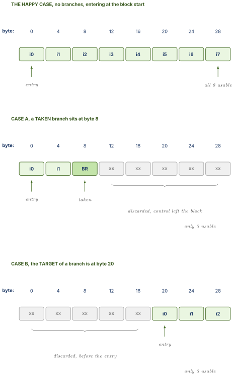
Estimate the average. If the entry point into a block is uniformly distributed across the 8 positions, the expected number of instructions from the entry to the end of the block is
and that is before accounting for a taken branch cutting it shorter still. So a fetch unit advertised as 8-wide delivers something under 4.5 instructions per cycle on branchy code. The back end can be as wide as you like and it will starve.
6.2 One taken branch per cycle
A second and independent limit. The fetch unit produces one next-fetch-address per cycle, so it can follow at most one taken branch per cycle.
That caps throughput directly. On code with a taken branch every 4 instructions, which is common in branch-dense code such as a parser or an interpreter, fetch cannot exceed 4 instructions per cycle regardless of block size, decoder count, or back-end width.
Some modern designs predict two taken branches per cycle, which requires the predictor to produce two independent predictions and the cache to service two non-contiguous reads in one cycle. Both are expensive, and it is a good illustration of how front-end bandwidth is bought in small, costly increments.
6.3 Decode width, and the genuine AArch64 advantage
Now the ISA matters, and this is one of the few places where an architectural difference has an unambiguous microarchitectural consequence.
AArch64. Every instruction is exactly 4 bytes and 4-byte aligned. Given a 32-byte block, the instruction boundaries are at bytes 0, 4, 8, 12, 16, 20, 24, and 28. Known with zero logic, before a single bit is examined. All 8 decoders start in parallel in the first cycle.
x86-64. Instructions are 1 to 15 bytes long. To know where instruction 2 starts, you must first determine instruction 1's length, which requires parsing any prefixes, then the opcode, then a ModRM byte, then possibly a SIB byte, then working out displacement and immediate sizes from those. That is inherently serial, and finding 8 boundaries naively means 8 sequential steps.
Three mitigations exist, and all three are expensive.
Brute-force parallel length decoding speculatively computes a length starting at every byte offset in the window, so a 32-byte window needs 32 length decoders plus a selection network to keep the ones that turn out to be real boundaries. Pre-decode bits stored alongside lines in the instruction cache mark the boundaries found the first time a line was decoded, paying the serial cost once. And the micro-op cache in 6.4 sidesteps decode entirely on a hit, which is a large part of why x86 designs invested in it first.
The consequence shows up in published decode widths. Apple's cores are reported to decode 8 instructions per cycle, while contemporary x86 designs sit at 4 to 6 and reach higher only through the micro-op cache path. That is a real, defensible advantage of a fixed-length encoding, and it is a reasonable thing to bring up unprompted in an interview.
6.4 The micro-op cache
Cache the decoded micro-operations instead of the raw instruction bytes, keyed by the address of the block they came from. On a hit, fetch and decode are skipped entirely and micro-ops are delivered straight to rename.
Three separate wins, and they are usually conflated.
Latency. Hitting in the micro-op cache removes several pipeline stages from the front end. That shortens in the formula from 1.3, which reduces the misprediction penalty on every branch in the resident code. A structure sold as a bandwidth feature is quietly also a prediction-cost feature.
Bandwidth. The micro-op cache is organized by the instruction stream, not by memory alignment. It stores the micro-ops that actually execute in the order they execute, so the fetch-alignment waste from 6.1 largely disappears on a hit.
Power. Instruction decode is a substantial fraction of front-end power, overwhelmingly so on x86. On a micro-op cache hit the entire decode cluster can be clock gated off, which is a direct application of Power Fundamentals and Clock Gating.
The costs are real too. It is another cache with its own capacity limits and its own misses, code that does not fit thrashes it, and it needs careful invalidation on self-modifying code and on remapping of code pages.
Note the asymmetry this creates between ISAs. For AArch64, the power argument is much weaker because fixed-length decode is cheap, and the bandwidth argument is weaker because alignment costs less when boundaries are free. Apple's cores are not reported to use a large micro-op cache in the way x86 designs do, and that is a direct downstream consequence of the encoding, not an arbitrary design preference.
6.5 The loop buffer
The narrowest and cheapest structure here, and almost purely a power play.
When the machine detects that it is executing a small loop, say under 64 micro-ops, it captures the loop body in a tiny buffer and replays it from there. Then fetch, the branch predictor, the BTB, and decode are all clock gated off for the duration.
Count what that saves on a 20-instruction loop running 10,000 times. Without the buffer, the machine performs 10,000 executions worth of instruction cache reads, BTB lookups, predictor table lookups, and 200,000 instruction decodes. With the buffer, it performs one pass worth and then shuts the entire front end down. There is a bandwidth benefit too, since the taken-branch limit from 6.2 no longer applies to the loop back-edge, but the reason it exists is power.
6.6 Fusion, seen from the front end
Out of Order Execution section 7.6 covered fusion from the back end's perspective, where it reduces pressure on quadratic structures. From the front end it does something else. It raises effective width without widening anything.
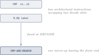
A machine that decodes 8 instructions and renames 6 micro-ops per cycle looks unbalanced. With compare-and-branch fusion firing on a couple of pairs in a typical block, 8 instructions become 6 micro-ops, and the two stages match exactly. The front end delivers 8 instructions worth of program per cycle through a 6-wide rename.
Two practical constraints worth knowing. The fusible pair must be adjacent, so a compiler that schedules an unrelated instruction between the compare and the branch destroys the opportunity. And the pair must fall in the same fetch block, so a fusible pair straddling a 32-byte boundary does not fuse. Both are reasons that measured fusion rates are lower than the theoretical opportunity count.
6.7 Decoupling, the fetch target queue, and overriding predictors
The last structural idea, and the one that ties the front end together.
The problem. If the branch prediction unit and the fetch unit run in lockstep, they share each other's stalls. When the instruction cache misses, the predictor stalls too even though it had plenty of work it could have done. And when the miss returns, the predictor starts cold from where it stopped.
The fix. Separate them with a queue. The branch prediction unit runs on its own, generating a stream of predicted fetch addresses and pushing them into a fetch target queue. The fetch unit pops addresses from the FTQ whenever it is ready.
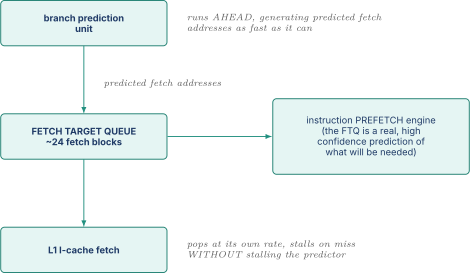
Three benefits, and the second one is the least obvious and the most valuable.
The predictor runs ahead by many blocks, so an instruction cache miss no longer stops prediction.
The contents of the FTQ are a genuine, high-confidence list of the instruction addresses the machine is about to need. That makes the FTQ the ideal driver for instruction prefetch. This is called fetch-directed instruction prefetching, and it is the most accurate instruction prefetch mechanism known, because unlike a data prefetcher it is not guessing a pattern, it is reading the machine's own plan. If the FTQ runs 10 blocks ahead and an L1 instruction miss costs 15 cycles, the prefetch was issued long enough ago to cover it.
And prediction and fetch no longer need the same latency. That last point enables something important. A full TAGE-SC-L with four tagged tables, long history hashes, a statistical corrector, and a loop predictor cannot produce a prediction in one cycle at a high clock frequency. Decoupling lets the predictor take two or three cycles.
The standard arrangement is an overriding predictor. A small fast predictor, often a simple bimodal or a small gshare plus the L1 BTB, produces a prediction in one cycle with zero bubble. The large slow predictor produces its answer two or three cycles later. If they agree, nothing happens and the fast path was free. If they disagree, the slow one wins and the machine pays a small two or three cycle bubble rather than the full 16-cycle misprediction penalty. Since they agree most of the time, the average cost is tiny and the accuracy is that of the big predictor.
07.Part 7, the whole front end, assembled
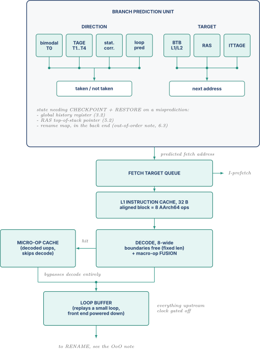
Read the diagram as answering the two failure modes from 1.2. The whole left-to-right top row exists to prevent correctness failures. The whole vertical stack below the FTQ exists to prevent bandwidth failures. The FTQ is where the two halves meet, and it is the only structure that helps both.
08.Part 9, check yourself
Answer out loud, in full sentences, as if an interviewer asked. If you cannot, reread the section named.
- Compute the added CPI at 20 percent branches, a 16-cycle penalty, and accuracy of 99, 95, and 90 percent. Against a base CPI of 0.2, what does that say about design priorities? (1.3)
- Why are branch predictor accuracy and reorder buffer size the same design decision seen from two ends? (1.3, and Out of Order Execution section 4.6)
- Where do the 16 penalty cycles physically come from, and give a case where the real penalty is far larger than the pipeline depth. (1.4)
- What accuracy does backward-taken-forward-not-taken reach, and what does that accuracy do to a wide out-of-order machine? (2.1)
- Trace a one-bit predictor through a 10-iteration loop. Why does it mispredict twice, and which of the two errors is avoidable? (2.2)
- Draw the two-bit saturating counter state diagram from memory, mark the prediction boundary, and explain why the same loop now mispredicts only once. (2.3)
- Why two bits and not three? (2.3)
- Give a code example that a per-branch predictor can never get right, tabulate why, and show how a two-bit global history fixes it exactly. (3.1, 3.2)
- Why must the global history register be updated speculatively, and what does that force you to build? Name the other two structures needing the same thing. (3.2, 5.2)
- Explain gshare in one sentence. With a fixed 12-bit index budget, why is XOR better than concatenation? (3.4)
- Classify the three kinds of aliasing and estimate how many colliding pairs you expect from 500 branches in a 4096-entry table. (3.5)
- In a tournament predictor, under what condition does the chooser update, and why not otherwise? (3.6)
- Why is any single history length wrong, and why are TAGE's history lengths geometric rather than evenly spaced? (4.1, 4.2)
- What do the tags in TAGE accomplish that a bigger untagged table cannot? (4.3)
- Work a 4-bit perceptron prediction and one training update by hand. What class of branch can it never learn, and why do tables get that case for free? (4.5)
- Why is a return address stack far more accurate than a BTB for returns, and what are its three failure modes? (5.2)
- Why does an interpreter dispatch loop defeat a BTB, and how does ITTAGE fix it? (5.3)
- A machine fetches aligned 32-byte blocks. Derive the average number of usable instructions per fetch and explain the two effects that reduce it. (6.1, 6.2)
- Why can AArch64 start 8 decoders in parallel immediately while x86 cannot, and name two things x86 designs do about it? (6.3)
- What three separate things does a micro-op cache buy, and why does an AArch64 design need it less than an x86 design? (6.4)
- What does decoupling the predictor from fetch enable, and why does it make fetch-directed instruction prefetch better than any data prefetcher? (6.7)
09.Part 10, related notes
- Out of Order Execution for the machine this feeds, the checkpoint and recovery mechanism the GHR and RAS reuse, and why window size tracks predictor accuracy
- CPU Foundations Pipeline and Hazards for pipeline depth, the CPI formula, and where the misprediction penalty comes from
- Cache Organization and Prefetching for the instruction cache the front end reads and for how fetch-directed prefetch compares with data prefetching
- Power Fundamentals and Clock Gating for the gating that makes the loop buffer and micro-op cache worth building, which is your strongest connection to this material
- SRAM Arrays and ECC for the arrays every predictor structure is built from, and for the argument about which of them need protection
- Modern Branch Predictors for the vault's deeper treatment of TAGE and perceptron
- Frontend Bandwidth for fetch alignment, decode, and the micro-op cache in more depth
- Project: A Branch Predictor Evaluator to build gshare, perceptron, and TAGE-SC-L and measure them, which is the thing that closes the gap in Part 8