Part IV·Memory Hierarchy·Chapter 37 of 66

Part IVMemory Hierarchy

Cache Fundamentals

August 3, 2026·29 min read·advanced

The memory wall of Chapter 36 makes one architectural response unavoidable. A processor that pays full DRAM latency on every memory access cannot keep its pipeline fed. The standard response is to place a small fast memory near the processor that holds the data the program is currently using and serve most accesses from that memory. The mechanism is the cache. This chapter develops cache design from first principles, starting with a single example, building up to the address decomposition that all cache designs share, and then surveying the three organizational families (direct-mapped, set-associative, fully associative) and the policies that govern how stores propagate through the hierarchy.

The treatment is concrete throughout. Every concept is introduced with a worked numerical example before any abstract definition. The reader who follows the worked examples will be able to compute hit-or-miss outcomes for any sequence of loads on a direct-mapped or set-associative cache by the end of the chapter.

01.A Concrete Cache

Imagine the simplest possible useful cache. It holds 4 lines, each of which is 16 bytes. Total capacity is 64 bytes. The cache sits between a 32-bit-addressed memory and a processor that issues loads and stores.

The cache must answer two questions on every access: is the data already here, and if so, where is it? To answer both questions quickly, the cache organizes its storage so the lookup is a constant-time operation. The standard mechanism is the address decomposition shown in Figure 1.

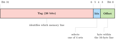
Figure 1. Address decomposition for a direct-mapped cache with 4 lines, each 16 bytes wide, on a 32-bit address space. The low 4 bits select a byte within the line. The next 2 bits select the line (index). The top 26 bits hold the tag.

The 4-bit offset selects which byte within the 16-byte line the access targets. The 2-bit index selects which of the 4 cache lines might hold the data. The top 26 bits form the tag that the cache stores alongside each line to confirm a match.

One Access Walked Through

A program issues lw t0, 0x4020. The address in binary is

Plain Text

0000 0000 0000 0000 0100 0000 0010 0000

The low 4 bits are 0000, so the access targets byte 0 of the line. The next 2 bits are 10, so the access targets set 2. The top 26 bits form the tag.

The cache controller does the following:

Select set 2 of the cache (one of four sets).
Read out the tag stored in set 2 and compare with the tag from the address.
If the tags match and the line is valid, return the 4 bytes starting at byte 0 of the line. This is a hit.
If the tags do not match, the access is a miss. Fetch the 16-byte line containing address 0x4020 from memory, install it in set 2 (evicting whatever was there), record the new tag, then return the requested word.

The entire lookup is one tag comparison and one data read, implemented as a single SRAM access plus a comparator. On a modern process this takes one or two clock cycles.

Why the Decomposition Works

The reason the address decomposition into tag, index, and offset is universal in cache design is that it lets the lookup happen in constant time. The index is a direct bit extraction. The tag is a direct bit extraction. The comparison is a fixed-width equality check. No address arithmetic is required, no search across multiple candidates, and no condition that depends on the data itself. Every cache architecture (direct-mapped, set-associative, fully associative) uses some variant of this decomposition. The only thing that changes is how many lines a given index selects.

02.Address Breakdown in General

The example above used a specific cache (4 lines, 16-byte lines, 32-bit address). The general rules are easy to derive. Define:

$A$ is the address width in bits.
$B$ is the line (block) size in bytes.
$S$ is the number of sets in the cache.
$W$ is the number of ways (lines per set). For a direct- mapped cache $W = 1$ , and for a fully associative cache $W$ equals the total number of lines.

The total cache data capacity in bytes is $S \times W \times B$ . The address decomposes as follows:

The offset is fixed by the line size. The index is fixed by the number of sets. The tag absorbs whatever is left of the address.

Example: a 32-KB L1 with 64-Byte Lines

A typical L1 data cache holds 32 KB of data, with 64-byte lines. Suppose it is 8-way set-associative. Then:

Total lines: $32768 / 64 = 512$ lines.
Number of sets: $512 / 8 = 64$ sets.
Offset width: $\log_2 64 = 6$ bits.
Index width: $\log_2 64 = 6$ bits.
Tag width (on a 64-bit address): $64 - 6 - 6 = 52$ bits.

Every cache lookup uses the bottom 12 bits of the address (6 for offset, 6 for index) and compares the top 52 bits against the tags in the selected set. The eight tag comparisons happen in parallel, typically completing in one to two cycles of pipelined logic.

03.Three Cache Organizations

The placement policy of a cache determines where a given memory address can be stored. Three policies cover all standard designs.

Direct-Mapped

A direct-mapped cache maps each memory address to exactly one cache location. The index field of the address selects that location. There is no choice: address $A$ can occupy only the line identified by index = (A >> log2(B)) mod S.

A direct-mapped cache is the simplest organization. The hardware needs one tag comparator and one data port. Lookups are fast, because there is no need to search multiple ways. The drawback is conflict misses. Two addresses that happen to share the same index field collide. The most recently accessed wins, and the other is evicted, even if the rest of the cache is empty.

Set-Associative

A set-associative cache with $W$ ways assigns each address to a set of $W$ lines. Any line in the set can hold the data. When the cache wants to install a new line in a set that is already full, a replacement policy decides which line to evict.

The hardware cost is roughly proportional to the associativity. A 4-way cache needs four tag comparators and four data ports per set. A 16-way cache needs sixteen. Beyond about 8-way, the area and energy cost of the extra comparators usually outweighs the hit- rate benefit, and designs hold associativity in the 4-to-16 range.

Fully Associative

A fully associative cache treats the entire cache as a single set. Any address can occupy any line. The lookup must compare the tag against every line in the cache, which requires $N$ comparators for an $N$ -line cache. This is expensive, so fully associative organizations are used only for small structures (the TLB, victim caches) where $N$ is at most a few dozen.

A fully associative cache has no conflict misses by definition. Its only misses are compulsory (the line has never been seen before) or capacity (the working set is larger than the cache). The table below summarizes the tradeoffs.

Table 1. Comparison of cache organizations. Conflict-miss column shows whether the organization is vulnerable to conflict misses. Hit time is approximate in pipelined logic.

Organization	Tag comparators	Conflict misses	Hit time
Direct-mapped	1	yes	1–2 cycles
2-way set-associative	2	rare	2–3 cycles
4-way set-associative	4	very rare	2–3 cycles
8-way set-associative	8	negligible	3–4 cycles
Fully associative (small)	$N$	none	3–5 cycles

Why Higher Associativity Has Diminishing Returns

The intuition that "more associativity always helps" is correct in the limit (a fully associative cache cannot conflict-miss), but the marginal benefit shrinks rapidly. Empirically, going from direct-mapped to 2-way cuts the conflict-miss rate by about half. Going from 2-way to 4-way cuts the remaining conflict misses by about half again. Going from 4-way to 8-way provides only a modest further improvement, and going past 8-way rarely justifies the area and energy cost. Hill and Smith documented this pattern in 1989, and it has held across decades of cache designs [1].

04.Hits, Misses, and the Three Cs

Every cache miss falls into one of three categories. Mark Hill named these categories the three Cs in his 1987 thesis [2], and they remain the standard taxonomy for analyzing cache behavior.

Compulsory Misses

A compulsory miss (also called a cold miss) occurs the first time a cache line is referenced. The line has never been in the cache before, so the lookup must miss regardless of cache size or associativity. The only way to eliminate compulsory misses is to fetch the line before the program asks for it, which is the job of prefetching (Chapter 40).

Compulsory misses dominate at the very start of a program’s execution. As the working set warms up, capacity and conflict misses take over. For long-running programs, compulsory misses are typically the smallest of the three categories.

Capacity Misses

A capacity miss occurs because the program’s working set exceeds the cache’s capacity. A line that was in the cache got evicted to make room for another line, and the evicted line is later referenced again.

Capacity misses scale with working-set size. A program with a 20 KB working set fits in a 32 KB cache and has zero capacity misses. The same program with a 64 KB working set spills out of the cache. The miss rate jumps the moment the working set crosses the cache boundary.

Conflict Misses

A conflict miss is a miss that would have been a hit in a fully associative cache of the same total size. It happens because multiple hot lines map to the same set, and the limited associativity forces eviction.

Conflict misses are sensitive to the address pattern, not just the working-set size. A loop that strides through addresses spaced exactly one set-stride apart hits every line in the same set, causing a storm of conflict misses. A loop that strides through addresses that distribute across sets evenly suffers no conflict misses at all.

Decomposing a Miss Rate

The three Cs are independent dimensions, and a workload’s miss rate can be decomposed accordingly. Figure 2 shows the canonical shape of miss rate as cache size varies, with each component contributing differently.

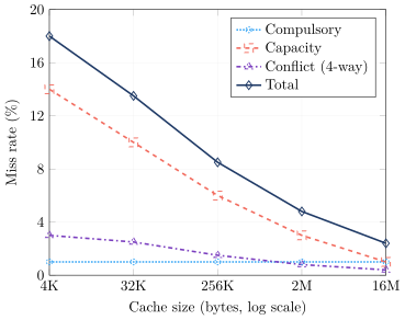
Figure 2. Typical three-C decomposition of cache miss rate as a function of cache size for a 4-way set-associative cache. The compulsory rate is flat. The capacity rate drops as the cache grows. The conflict rate also drops, but more slowly. Source: Hill and Smith� , generalized.

The decomposition is helpful because each component responds to different design changes. Compulsory misses respond only to prefetching. Capacity misses respond to larger caches. Conflict misses respond to higher associativity. A designer choosing how to spend a fixed area budget can ask which component dominates and target that component first.

05.Replacement Policies

When a new line is brought into a set that is already full, the cache must choose which existing line to evict. The replacement policy makes that choice. For set-associative caches, three policies cover the standard designs.

LRU: Least Recently Used

Least recently used (LRU) replacement evicts the line in the set that has gone the longest without a reference. The intuition is that lines used recently are likely to be used again soon (temporal locality), and lines that have not been touched recently are likely the coldest.

True LRU is expensive to implement. For an $N$ -way set, the cache must maintain an ordering of the $N$ lines, updated on every access. The ordering itself needs $\log_2(N!)$ bits per set to encode, which for $N = 8$ is 16 bits and grows quickly. The update logic is also non-trivial. Real designs typically approximate LRU with simpler schemes (the subject of Chapter 38, which covers tree-PLRU and MRU-based approximations).

Example: LRU Walk-Through

A 4-way set-associative set holds 4 lines, labeled A, B, C, D. The access sequence on this set is A, B, C, D, A, E, B, F. Show the LRU order after each access and identify which lines are evicted.

Solution. Track the order from most recent to least recent.

After A: [A] (A is MRU, set has 3 free ways).

After B: [B, A].

After C: [C, B, A].

After D: [D, C, B, A]. Set is full.

After A: [A, D, C, B]. A was already present, so promote to MRU.

After E: E enters and evicts the least recent, B. [E, A, D, C].

After B: B is not present, this is a miss. Evict C. [B, E, A, D].

After F: F is not present, this is a miss. Evict D. [F, B, E, A].

In total, 8 accesses with 7 misses and 1 hit. LRU correctly kept A across its second access. The three evictions matched the temporal- locality intuition.

FIFO: First In, First Out

FIFO replacement evicts the line that has been in the set longest, regardless of recent use. It is simpler than LRU because the state is a fixed pointer per set, not a full ordering. FIFO performs worse than LRU on most workloads, because it does not respect the recency intuition. It can also exhibit Belady’s anomaly, in which a larger cache produces a higher miss rate than a smaller cache on the same workload, a property that no anomaly-free policy can have.

Random

Random replacement evicts a randomly chosen line. It is the simplest policy to implement (one linear-feedback shift register per set generates the choice) and performs surprisingly close to LRU on most workloads. The correlation between recent use and future use is real but weak enough that a uniformly random choice is rarely much worse than LRU. Some designs deliberately use random replacement to defeat side-channel attacks that exploit deterministic eviction patterns.

Belady’s Optimal Algorithm

The theoretical lower bound on replacement-policy misses is Belady’s algorithm [3], which evicts the line whose next reference is farthest in the future. It is unimplementable in hardware because it requires knowledge of future references, but it serves as the benchmark against which real policies are measured. A typical workload’s LRU miss rate is within 10-20 percent of Belady’s. Random replacement is typically 30-50 percent worse than Belady’s.

06.Write Policies

Loads are simple: the cache either has the data or it does not. If it has the data, return the requested bytes. If not, fetch the line from below and return.

Stores are more interesting. A store updates a memory location. The cache must decide where to keep that update and when to propagate it to the level below. Two orthogonal choices govern write behavior: the propagation policy (write-through vs. write-back) and the allocation policy (write-allocate vs. no-write-allocate). The four combinations correspond to four design points.

Write-Through

A write-through cache propagates every store to the level below immediately. The cache stays up to date, but every store generates a write to memory or to the next-level cache. The lower level must absorb the write bandwidth.

The advantage of write-through is simplicity. The cache and the level below are always consistent. Eviction of a clean line costs nothing because the level below already has the latest value.

The disadvantage is write bandwidth. A program that performs heavy write-heavy workloads can saturate the link to the level below. Most modern designs use a write buffer, a small FIFO that queues outgoing writes so the processor does not have to stall waiting for each one to complete. The write buffer turns synchronous writes into asynchronous ones, decoupling the processor from the write bandwidth.

Write-Back

A write-back cache updates only its own copy of the line on a store and marks the line dirty. The dirty line is written to the level below when the cache evicts it, combining many updates into a single write.

The advantage is write traffic. A loop that repeatedly stores to the same address in a write-back cache generates one write to memory (when the line is evicted), not one per store. For a 64-byte line with 16 four-byte words touched by 100 stores each, that is a reduction of about 1600 writes to one.

The disadvantage is bookkeeping. Each line carries a dirty bit. On eviction, the cache must check the dirty bit and, if set, write the line back before installing the new line. The write-back can stall the eviction, which is why high-end caches separate the eviction from the writeback through a writeback buffer.

Write-Allocate

A write-allocate cache fetches the line on a store miss, just as it would on a load miss. The store then updates the in-cache copy. This is the natural pairing for write-back caches: the cache cannot mark a line dirty if it does not hold the line.

The cost is the extra fetch on store misses. A program that writes to many new locations without ever reading them (initializing a large buffer, for example) pays a full miss fetch for every cache line it touches, even though it has no need for the old contents. Some designs offer a non-temporal store instruction that bypasses the cache to avoid this cost.

No-Write-Allocate

A no-write-allocate cache on a store miss writes the value to the level below without bringing the line into the cache. This is the natural pairing for write- through caches: the store has to go to memory anyway, so there is no benefit to fetching the line into the cache.

The advantage is fewer fetches on write-heavy workloads. The disadvantage is that follow-up loads to the same line will miss, because the line is not in the cache.

The Four Combinations

The table below summarizes the four combinations and their typical use cases.

Table 2. Write policy combinations. The most common pairings in modern designs are write-back with write-allocate (for high- performance caches) and write-through with no-write-allocate (for caches close to a fast next level, like L1 with a fast L2 backing it).

Propagation	Allocation	Typical use
Write-back	Write-allocate	Modern L1, L2, L3. The best balance of write bandwidth and hit-rate behavior.
Write-through	No-write-allocate	Some L1 designs with a fast adjacent L2. The L2 absorbs the write traffic.
Write-back	No-write-allocate	Rare. Some inclusive cache designs use this for the LLC.
Write-through	Write-allocate	Uncommon. Has no clear advantage over the alternatives.

The dominant pairings on modern processors are write-back with write-allocate for caches that have substantial behind-the-cache miss penalty (L2, L3, and most L1 designs), and write-through with no-write-allocate for L1 designs that have a fast nearby L2.

07.Tag Storage and Total Cache Size

The cache stores tag bits, valid bits, and (for write-back caches) dirty bits in addition to the data. The metadata is not free, and the total cache size is the data size plus the metadata size.

Example: Total Size of a 32-KB L1

Consider a 32-KB 8-way set-associative L1 data cache with 64-byte lines on a 64-bit machine. Compute the total bits required for the metadata.

Solution.

Number of sets: $32768 / (64 \times 8) = 64$ sets.
Number of lines: 512.
Tag width: $64 - 6 - 6 = 52$ bits per tag.
Valid bit: 1 per line.
Dirty bit (if write-back): 1 per line.
Total metadata: $512 \times (52 + 1 + 1) = 512 \times 54 = 27{,}648$ bits $\approx 3.4$ KB.

The metadata adds about 10 percent to the cache’s storage budget. This overhead is typical for L1 designs. Larger caches with longer lines amortize the metadata over more data per tag, so the ratio drops. An L3 with 64-byte lines and 22-bit tags carries about 5 percent metadata overhead.

The metadata storage is part of the cache’s design budget. A 32-KB L1 is really about 35 KB of SRAM after metadata. This matters when comparing cache sizes across processors, because vendors quote the data size only.

08.Cache Behavior on a Code Sequence

To consolidate the chapter, walk through the cache behavior on a realistic code sequence. The following RV32I loop initializes an array of 256 integers to zero.

Array initialization loop

Riscv

li      t0, 0          # zero value
        la      t1, array      # base address (assume 256-byte aligned)
        li      t2, 256        # count
init:
        sw      t0, 0(t1)      # store zero
        addi    t1, t1, 4      # advance pointer
        addi    t2, t2, -1     # decrement counter
        bnez    t2, init       # loop until done

Assume a 32-byte direct-mapped L1 data cache with 8-byte lines. The cache has 4 lines. The array array starts at address 0x1000.

The first store writes to address 0x1000, which has offset 000, index 00, and a tag. The cache is cold, so this is a compulsory miss. The cache fetches the 8-byte line covering addresses 0x1000-0x1007 into set 0.

The second store writes to address 0x1004, which is in the same line. This is a hit. Likewise the line covers addresses 0x1000-0x1007, so the second store hits.

The third store writes to address 0x1008, which is the next line. Offset 000, index 01. This is a compulsory miss, fetching the line into set 1.

The pattern continues. Every other store is a compulsory miss, and the intervening store is a hit. The hit rate over the 256 stores is $256/2 = 128$ hits out of 256 stores, or 50 percent. Each cache miss costs the latency to fetch a 8-byte line from memory. Each hit costs only the L1 latency.

A larger line size would amortize the miss latency over more stores. With 64-byte lines (16 integers per line), one miss covers 16 stores, and the hit rate climbs to 15/16 = 93.75 percent. This is the spatial-locality benefit at the cache-line level.

09.Inclusive, Exclusive, and Hybrid Hierarchies

This chapter has treated a single cache in isolation. Real processors have two or three levels of cache, and the levels interact. The relationship between an upper level (closer to the processor) and a lower level (farther from the processor) can take three forms.

Inclusive. Every line in the upper cache is also present in the lower cache. The lower cache is a superset of the upper. This simplifies coherence: snoop traffic from other cores can check only the lower cache to determine whether a line is held by this core. The cost is that the lower cache duplicates data that the upper cache already holds.

Exclusive. A line is in either the upper cache or the lower cache, never both. This maximizes the effective storage (total capacity is the sum of the two), at the cost of more complex movement when lines transit between levels.

Non-inclusive non-exclusive (NINE). The two levels are independent. A line may be in both, in either, or in neither. This is the most common design point. Chapter 38 develops the tradeoffs in detail.

10.Looking Ahead

The next chapter develops the quantitative tools for analyzing cache performance: the average memory access time formula, multi-level cache analysis, and the more sophisticated replacement approximations that real designs use. The chapter after that surveys the advanced cache organizations (skewed-associative, way-prediction, sectored, and others) that modern high-performance designs deploy.

11.Worked Examples

Example: Hit-or-Miss Sequence

A 2-way set-associative cache has 4 sets and 16-byte lines. Initially empty. The CPU issues loads to addresses 0x000, 0x040, 0x080, 0x000, 0x040. Identify hit or miss for each.

Solution. Cache has 4 sets, 16-byte lines, so offset is 4 bits, index is 2 bits. Index of 0x000 is bits 4-5 of 0x000 = 00 = set 0. Index of 0x040 is bits 4-5 of 0x40 = 00 = set 0. Index of 0x080 is bits 4-5 of 0x80 = 00 = set 0. All three addresses map to set 0.

Access 1 (0x000): miss. Set 0 has [tag for 0x000].

Access 2 (0x040): miss. Set 0 has [tag for 0x000, tag for 0x040].

Access 3 (0x080): miss (set 0 is full, so LRU evicts 0x000). Set 0 has [tag for 0x040, tag for 0x080].

Access 4 (0x000): miss (evicted on access 3). Set 0 has [tag for 0x080, tag for 0x000] after LRU eviction of 0x040.

Access 5 (0x040): miss (evicted on access 4). Set 0 has [tag for 0x000, tag for 0x040].

All five accesses miss. The set-associative cache absorbed nothing because all three addresses fall in the same set. A 4-way cache would have hit on access 4 and 5.

Example: Allocation Policy Tradeoff

A program initializes a 1 MB buffer by writing zero to every byte. The cache is 32 KB with 64-byte lines and is empty. Compare the miss-fetch traffic for write-allocate vs no-write-allocate.

Solution. Write-allocate: 1 MB / 64 B = 16,384 cache lines. Each first store to a line is a miss that fetches the (uninitialized) line from memory. Total fetch traffic: $16{,}384 \times 64~\text{B} = 1$ MB.

No-write-allocate: Stores that miss bypass the cache and write directly to memory. No fetches. Fetch traffic: 0.

For a pure initialization workload, no-write-allocate saves 1 MB of fetch traffic. The cost is that subsequent reads of the buffer miss the cache, requiring fetches at that point.

A non-temporal store hint (or RISC-V’s cbo.zero) bypasses this tradeoff: it tells the cache to skip the fetch and treat the line as zero, which is what the program wants.

12.Exercises

Exercises

Tag-index-offset. A cache holds 64 KB of data with 128-byte lines and is 16-way set- associative. On a 64-bit address space, compute the width of the tag, index, and offset fields.
Capacity vs conflict. A direct-mapped cache of size $C$ has miss rate $M_D$ . A fully associative cache of size $C$ has miss rate $M_F$ . Sketch how the miss rate of an $N$ -way set-associative cache transitions from $M_D$ at $N = 1$ to $M_F$ at $N = C / B$ . On what empirical observation does the rule of thumb "double the associativity, halve the conflict miss rate" rest?
Address mapping. For a 4 KB 2-way set-associative cache with 16-byte lines, identify which set holds each of the following addresses: 0x1000, 0x1080, 0x1200, 0x2000.
LRU ordering. A 4-way set has access sequence A, B, A, C, B, D, C, E. Show the LRU order after each access and identify the evictions.
FIFO and Belady’s anomaly. A FIFO 3-line cache and a FIFO 4-line cache run the access sequence 1, 2, 3, 4, 1, 2, 5, 1, 2, 3, 4, 5. Count misses for each. Show that the larger cache has more misses (Belady’s anomaly).
Write-back metadata. A 1 MB 8-way set-associative L2 cache has 64-byte lines, dirty bits, and 26-bit tags. Compute the metadata storage as a percentage of the data storage.
Write-buffer sizing. A processor at 3 GHz commits at most 2 stores per cycle on a worst-case mix. The link to L2 sustains 16 GB/s. How many entries does the write buffer need to absorb a 100-cycle burst of stores without stalling the pipeline?
Three-C decomposition. A workload misses 1 percent at a 64 KB 4-way cache, 0.6 percent at a 64 KB 8-way cache, and 0.5 percent at a 64 KB fully associative cache. Estimate the compulsory, capacity, and conflict components at 4-way associativity.
Line size selection. A program touches one new 8-byte object per loop iteration and strides linearly through memory. The cache offers 32-byte or 128-byte lines. Which is better for hit rate? For bandwidth utilization? Discuss the tradeoff.
Associativity ceiling. Why do modern designs rarely use associativity above 16, even for the L3 where conflict misses can be costly?
Replacement under cycle pressure. A 16-way set with true LRU requires $\log_2(16!) \approx 45$ bits of ordering state. Propose a simpler approximation that uses about 4 bits per line. What property of LRU does the approximation preserve?
Write-back transit cost. A line evicted from a write-back L1 must be written back to L2. On a typical processor, the writeback traffic adds 1-3 percent to L2 bandwidth. Why is this acceptable while a write-through L1 generating 10-20 percent more L2 traffic is not?
Compulsory miss elimination. What is the only architectural technique that can eliminate compulsory misses without increasing cache size?
Index bit selection. Most caches index using the low-order bits of the address (after the offset). Some research designs use a hash of high and low bits. What is the motivation for hashing? When does it help?
Cache pollution. A streaming workload reads a 100 MB array exactly once. The L2 is 1 MB. What happens to the L2’s existing contents? Does it matter for performance, given that the streaming data is never re-read?

References

[1]Hill, Mark D. and Smith, Alan Jay (1989). “Evaluating Associativity in CPU.” IEEE Transactions on Computers, 38(12), pp. 1612--1630. doi:10.1109/12.42289
[2]Hill, Mark D. (1987). “Aspects of Cache Memory and Instruction Buffer Performance.”
[3]Belady, L\'aszl\'o A. (1966). “A Study of Replacement Algorithms for a Virtual-Storage Computer.” IBM Systems Journal, 5(2), pp. 78--101. doi:10.1147/sj.52.0078

Book mode

	li t0, 0 # zero value
	la t1, array # base address (assume 256-byte aligned)
	li t2, 256 # count
	init:
	sw t0, 0(t1) # store zero
	addi t1, t1, 4 # advance pointer
	addi t2, t2, -1 # decrement counter
	bnez t2, init # loop until done