Part IV·Memory Hierarchy·Chapter 38 of 66

Part IVMemory Hierarchy

Cache Performance Analysis

August 3, 2026·24 min read·advanced

The cache organizations of Chapter 37 are the mechanism. Performance analysis is what tells the architect whether the mechanism is doing its job. This chapter develops the quantitative tools. The average memory access time formula compresses the behavior of a single cache into one number. Its multi-level extension does the same for the modern two- and three-level hierarchies. Inclusion policy governs how those levels relate. Replacement-policy approximations let designs ship full associativity without the area of true LRU.

The chapter is calculation-heavy. Most sections carry a worked calculation, and the chapter closes with a set of worked examples that the reader can verify with paper and pen. The expectation by the end is that a reader given the parameters of a cache hierarchy (sizes, associativities, latencies, miss rates) can predict effective CPI without consulting a simulator.

01.Average Memory Access Time

The headline metric for a cache is its average memory access time (AMAT). It compresses the cost of a memory reference into a single expected value, weighting the fast hit case by its probability and the slow miss case by its.

The reasoning is straightforward. Every access pays $t_{\text{hit}}$ to look up the cache, regardless of whether the lookup hits or misses. On a miss, which occurs with probability $m$ , the access also pays the miss penalty to fetch the line from the level below. The expected total is the hit time plus the miss-weighted penalty.

A First Example

Consider an L1 cache with a 4-cycle hit time, a 5-percent miss rate, and a 200-cycle miss penalty (to fetch from DRAM, ignoring any L2 or L3 for the moment).

$\text{AMAT} \;=\; 4 + 0.05 \times 200 \;=\; 4 + 10 \;=\; 14~\text{cycles}.$

A naive reading of the cache parameters might suggest that each access takes 4 cycles when it hits and 204 cycles when it misses. That is true per access. But for a stream of many accesses, the expected cost is 14 cycles. A program with one million memory references will spend about $14 \times 10^{6}$ cycles on memory, regardless of how those references happen to break across hits and misses (in the limit of large $N$ ).

Why AMAT Matters More Than Hit Rate

A naive comparison of caches by hit rate alone is misleading. AMAT combines hit rate and miss penalty into a single number that predicts performance. Consider two designs:

Cache A: 4-cycle hit, 4-percent miss rate, 200-cycle penalty. AMAT $= 4 + 0.04 \times 200 = 12$ cycles.
Cache B: 6-cycle hit, 3-percent miss rate, 200-cycle penalty. AMAT $= 6 + 0.03 \times 200 = 12$ cycles.

Both have identical AMAT. Cache B has a better hit rate but a slower hit time. The two effects cancel exactly. A designer choosing between them would need to consider second-order effects (power, area, downstream pipeline behavior) rather than the headline performance number, because the headline numbers agree.

02.Multi-Level Caches

Real processors have two or three levels of cache between the processor and DRAM. The AMAT formula extends naturally. The miss penalty for the upper level is itself an AMAT of the next level down. Recursive substitution gives the full hierarchy.

For three levels:

$\text{AMAT} \;=\; t_{\text{L1}} + m_{\text{L1}} \cdot \bigl( t_{\text{L2}} + m_{\text{L2}} \cdot ( t_{\text{L3}} + m_{\text{L3}} \cdot t_{\text{DRAM}}) \bigr).$

The structure is layered. Every access pays the L1 hit time. The fraction that miss L1 pays the L2 hit time as well. Of those, the fraction that miss L2 pays the L3 hit time, and so on. The miss penalty at the bottom of the hierarchy is the time to reach DRAM.

Concrete Example

A typical modern desktop processor has:

L1: 32 KB, 4 cycles, 5-percent miss rate.
L2: 1 MB, 12 cycles, 15-percent local miss rate.
L3: 24 MB, 40 cycles, 30-percent local miss rate.
DRAM: 200 cycles.

Compute AMAT:

$\text{AMAT} = 4 + 0.05 \cdot \bigl(12 + 0.15 \cdot (40 + 0.30 \cdot 200)\bigr).$

Work outward:

$40 + 0.30 \times 200 = 40 + 60 = 100.$

$12 + 0.15 \times 100 = 12 + 15 = 27.$

$4 + 0.05 \times 27 = 4 + 1.35 = 5.35~\text{cycles}.$

The full three-level hierarchy delivers an average memory access time of 5.35 cycles. Without the L2 and L3, the same L1 would deliver $4 + 0.05 \times 200 = 14$ cycles. The lower-level caches reduce the effective access time by more than a factor of 2.5.

03.Local Versus Global Miss Rates

The miss rate of a lower-level cache can be reported in two ways, and the two are easy to confuse.

The local miss rate of L2 is the fraction of accesses that reach L2 and miss. In the previous example, 15 percent of L2 accesses missed. The local rate is the right number to plug into the AMAT formula.

The global miss rate of L2 is the fraction of total memory references issued by the processor that miss in L2. The total references include those that hit in L1 and never reached L2. To convert, multiply by the L1 miss rate:

$m_{\text{L2,global}} \;=\; m_{\text{L1}} \cdot m_{\text{L2,local}}.$

In the example, $m_{\text{L2,global}} = 0.05 \times 0.15 = 0.0075$ , or 0.75 percent. Only 0.75 percent of total memory references miss in L2.

Why the Local Rate Looks High

A 15-percent local L2 miss rate sounds alarming. The intuition is wrong. The L2 only sees accesses that L1 already failed to absorb, which are the harder cases by construction. The L1 filtered out all the easy accesses. The L2 is seeing the residual, which has worse locality than the original stream. A 15-percent miss rate on that filtered stream corresponds to only 0.75 percent of total references. In global terms the L2 is doing excellent work.

04.From AMAT to Effective CPI

AMAT is the cost per memory reference. To convert to CPI, account for the fraction of instructions that are memory references.

where $\text{CPI}_{\text{base}}$ is the CPI assuming all memory accesses are free (one cycle each, hitting L1 in the same cycle as the instruction), $f_{\text{mem}}$ is the fraction of instructions that are loads or stores, and the $(\text{AMAT} - 1)$ term subtracts the one cycle of memory access already baked into the base CPI.

A Workload Walkthrough

A workload has base CPI of 1.0, with 30 percent of instructions being loads or stores. The cache hierarchy delivers AMAT of 5.35 cycles (from the previous section). Effective CPI:

$\text{CPI}_{\text{eff}} = 1.0 + 0.30 \times (5.35 - 1) = 1.0 + 0.30 \times 4.35 = 1.0 + 1.305 = 2.305.$

The processor spends 1.0 cycles per instruction on compute and 1.305 cycles on memory waits, for a total of 2.305 cycles per instruction. More than half the runtime is memory.

If the L1 hit rate degrades to 90 percent (from 95 percent), recompute. Each step amplifies through the hierarchy:

$40 + 0.30 \cdot 200 = 100.$ $12 + 0.15 \cdot 100 = 27.$ $4 + 0.10 \cdot 27 = 4 + 2.7 = 6.7.$ $\text{CPI}_{\text{eff}} = 1.0 + 0.30 \cdot (6.7 - 1) = 1.0 + 1.71 = 2.71.$

A 5-percentage-point reduction in L1 hit rate increased CPI from 2.305 to 2.71, an 18-percent slowdown. The cache hierarchy is sensitive to small changes in L1 behavior because every L1 miss propagates downstream.

05.Inclusion, Exclusion, and NINE

When a processor has multiple cache levels, the relationship between an upper-level line and the lower level determines coherence behavior, capacity behavior, and replacement behavior. Three policies are common.

Inclusive

An inclusive hierarchy guarantees that every line in an upper level is also present in the lower level. The L3 holds a copy of every line in any L2, and each L2 holds a copy of every line in its L1. The lower levels are supersets of the upper.

The advantage is coherence. To check whether this core holds a given line (for example, in response to a snoop from another core), the coherence logic needs to consult only the L3. If the line is not in the L3, it is not in this core’s L1 or L2 either, by the inclusion property. The lower levels serve as a directory.

The disadvantage is capacity. The total effective storage of an inclusive L1+L2+L3 hierarchy equals the size of the largest level, not the sum. A core with a 32 KB L1, a 1 MB L2, and a 32 MB L3 has 32 MB of effective storage, not 33.032 MB. The duplication is overhead.

Inclusion also constrains replacement. When the L3 evicts a line, it must back-invalidate any L1 or L2 copies. This back-invalidation traffic is a real cost.

Exclusive

An exclusive hierarchy keeps each line in exactly one level. A line in L1 is not in L2 or L3. When the L1 evicts a line, the line moves to the L2 (rather than being discarded). When the L2 evicts a line, it moves to the L3.

The advantage is capacity. The effective storage is the sum of all levels. A 32 KB L1 + 1 MB L2 + 32 MB L3 exclusive hierarchy provides 33.032 MB of effective storage.

The disadvantage is movement. Every L1 eviction moves a line. Every L2 eviction moves a line. The bandwidth between levels can be substantial. Coherence is also harder because the snoop logic must check every level.

NINE (Not-Inclusive Non-Exclusive)

The dominant modern design point is non-inclusive non-exclusive. There is no enforced relationship between levels. A line can be in both L1 and L2, in only one, or in neither. The cache controllers operate independently.

The advantage is design simplicity. Each level has its own replacement policy and its own behavior. No back-invalidation on eviction. No mandatory movement on eviction. The hardware is simpler than either pure inclusive or pure exclusive.

The disadvantage is coherence overhead. A snoop must check every level. Most processors solve this through a directory or through restricted snoop traffic.

Comparing the Three

Table 1. Comparison of inclusion policies. Effective storage is the total capacity available for unique lines. Back-invalidation is the L3-to-L1 traffic when a lower-level eviction forces an upper-level eviction. Snoop scope is how many levels a coherence query must check.

Policy	Effective storage	Back-invalidation	Snoop scope
Inclusive	= L3 size	yes	L3 only
Exclusive	L1 + L2 + L3	no	all levels
NINE	between L3 and sum	no	all levels

Modern processors vary in their choice. Intel typically uses inclusive L3 in older Xeon designs (Westmere through Broadwell) and switched to NINE starting with Skylake-X. AMD Zen uses NINE throughout. ARM’s Cortex-A77 and later use NINE. Apple’s M-series chips are believed to use NINE based on public reverse-engineering work, though Apple does not publish microarchitecture details.

06.Victim Caches

A victim cache is a small fully- associative buffer that catches lines evicted from the main cache, giving them a second chance. The idea is due to Jouppi [1], who observed that a small set of recently-evicted lines often gets re-referenced soon after eviction, particularly in caches with low associativity.

A typical victim cache holds 4 to 16 lines. On an access, the processor probes both the L1 and the victim cache in parallel. If the L1 misses and the line is in the victim cache, swap it back into the L1 (evicting the L1 line into the victim cache). The lookup avoids the L2 access entirely.

The benefit is largest for direct-mapped or low-associativity L1 designs, which suffer the most conflict misses. A direct-mapped L1 with a 4-entry victim cache often achieves miss rates close to a fully associative cache of the combined size. The hardware cost is small: a 4-line fully-associative buffer is cheap.

Modern high-associativity L1 designs typically dispense with the victim cache because the L1 already absorbs most of the conflicts. Victim caches reappear at the L3 in some designs, where they buffer recent L3 evictions before the line is written back to memory.

07.Replacement Approximations

True LRU replacement requires $\log_2(N!)$ bits of state per set for an $N$ -way cache. For $N = 8$ this is 16 bits per set. For $N = 16$ it is 45 bits per set. The update logic to keep the ordering current on every access is also substantial. Real designs almost always use an approximation that captures most of the LRU benefit at a fraction of the storage and update cost.

Tree-PLRU

Tree-PLRU maintains a binary tree of bits that tracks recency at each split of the set. For an $N$ -way set the tree has $N - 1$ internal nodes, each holding a single bit. The bit at a node indicates which half of the tree was most recently used.

Figure 1 shows a tree-PLRU for an 8-way set. On a hit, walk from the leaf for the hit line back to the root, setting each bit to point away from the hit half. On a miss that requires eviction, walk from the root following the bits in their current state. The leaf reached is the victim.

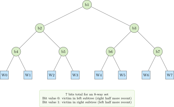
Figure 1. Tree-PLRU state for an 8-way set. Seven bits encode the binary tree. On a hit, walk from the hit leaf to the root, flipping each bit to point away. On a miss, walk from the root following the bits to the victim leaf.

Tree-PLRU is the dominant approximation in commercial designs. It matches true LRU within a few percent on most workloads, with roughly $\log_2 N$ the storage and trivial update logic. For $N = 8$ it uses 7 bits per set instead of 16. For $N = 16$ it uses 15 bits per set instead of 45.

NRU and MRU-Based

A not recently used (NRU) policy uses a single bit per line: 1 if the line has been used recently, 0 otherwise. On a hit, set the bit. On a miss requiring eviction, find any line with bit 0 and evict it. If all bits are 1, clear them all and try again.

NRU is even simpler than tree-PLRU. The state is $N$ bits per set instead of $N - 1$ . Update is trivial (set a single bit on each hit). The downside is that NRU loses ordering information: it distinguishes only recent from non-recent, not most-recent from second-most-recent. On workloads with strong recency, this can hurt hit rate by 1 to 3 percent compared with true LRU.

A variant of NRU called re-reference interval prediction (RRIP) encodes more state per line (typically 2 bits) and can match true LRU performance, sometimes exceeding it on scan-resistant workloads. Modern L3 designs in some processors use RRIP-style policies.

Pseudo-LRU and the Empirical Story

Empirically, the differences between tree-PLRU, NRU, RRIP, and true LRU rarely exceed 5 percent on AMAT for typical workloads. The choice of replacement policy is a second-order concern in modern cache design. The first-order concerns are cache size, associativity, and prefetching, all of which can change AMAT by tens of percent.

08.Bandwidth-Limited Versus Latency-Limited Behavior

AMAT measures latency. A different lens is bandwidth. A cache also has a sustained bandwidth limit, set by the number of ports, the line size, and the access cycle time. For workloads that saturate that limit, latency analysis under-predicts the cost of memory.

A 32-KB L1 with one read port that completes one access per cycle at 3 GHz delivers $3 \times 10^{9} \times 8~\text{B} = 24$ GB/s of read bandwidth (for 8-byte loads). A vectorized workload that issues two loads per cycle saturates the L1 port immediately and sees CPI bounded below by the port count.

Modern L1 designs typically offer 2 read ports and 1 write port, or some variant. The L2 might have 1 read port shared between instruction fetch and data load. The L3 has 1 port shared across all cores. Each level has its own bandwidth ceiling. AMAT analysis should be supplemented with bandwidth analysis when the workload is vector-heavy or memory-streaming.

09.A Full Workload Analysis

To consolidate the chapter, walk through a complete cache-hierarchy analysis for a hypothetical workload. The workload is a matrix multiplication of two 2048-element-square float32 matrices. Suppose the inner loop body resembles the following:

Matrix multiplication inner loop

for (int i = 0; i < N; i++) {
    for (int j = 0; j < N; j++) {
        float acc = 0.0f;
        for (int k = 0; k < N; k++) {
            acc += A[i][k] * B[k][j];
        }
        C[i][j] = acc;
    }
}

Each matrix is $2048 \times 2048 \times 4$ bytes $= 16$ MB. The total memory footprint of the three matrices is 48 MB.

Access Pattern

The inner loop reads A[i][k] and B[k][j] on every iteration. A[i][k] strides with $k$ , so it accesses 4 bytes apart sequentially (good spatial locality). B[k][j] strides with $k$ but holds $j$ constant, so it accesses $2048 \times 4 = 8192$ bytes apart (each B[k][j] for successive $k$ is on a different cache line).

Cache Behavior

The L1 is 32 KB. The row of A that the inner loop reads is 8 KB (2048 floats), fitting in L1. The 2048-element column of B is also 8 KB, but those elements live on 2048 different cache lines (8 KB of useful data spread across $2048 \times 64 = 128$ KB of cache footprint). The L1 cannot hold this column.

So the access to A[i][k] hits in L1 (after warming). The access to B[k][j] misses L1, missing L2 (a given column is revisited only on the next $i$ iteration, by which time the $j$ loop has swept all 16 MB of B through the L2), and at best hits L3 (24 MB) after warming.

Quantitative AMAT

Suppose: L1 = 4 cycles, L2 = 12, L3 = 40, DRAM = 200. The workload has two memory references per inner-loop iteration: one to A (hits L1) and one to B (misses L1, L2, sometimes L3). For the A access, AMAT $= 4$ cycles. For the B access, apply the equation above with a 99-percent L1 miss rate, an 80-percent L2 local miss rate, and a 20-percent L3 local miss rate:

$\text{AMAT}_{\text{B}} \;=\; 4 + 0.99 \cdot \bigl(12 + 0.80 \cdot (40 + 0.20 \cdot 200)\bigr) \;=\; 4 + 0.99 \cdot 76 \;\approx\; 79.2~\text{cycles}.$

Average AMAT over the two references: $\approx (4 + 79.2)/2 \approx 41.6$ cycles per reference. With a base CPI of 1 and 67 percent memory references (each inner-loop iteration has 2 loads and 1 FMA), effective CPI is roughly $1 + 0.67 \times (41.6 - 1) \approx 28$ .

The matrix multiplication runs 30 times slower than its compute peak. The cause is the column access to B, which has miserable locality.

Why Blocking Helps

The standard optimization is to block the inner loops to keep a subblock of B resident in L1. Replace the inner loop with a triple loop over blocks of size $B \times B$ . Choose $B$ so that the blocks fit in L1 ( $B^2 \cdot 4 \leq 32~\text{KB}$ , so $B \leq 90$ ). The blocked version restores locality. The AMAT drops to nearly L1 hit time, and the matrix multiplication runs at nearly compute peak. Blocking is one of the most important compiler and library optimizations precisely because it changes AMAT by an order of magnitude.

10.Looking Ahead

The next chapter surveys cache techniques beyond the basic organization. Skewed associativity, way prediction, line buffers, sectored caches, compressed caches, cache bypass, and dead-block predictors are all techniques real high-performance designs deploy to push the AMAT formula’s components lower. The chapter after that, on prefetching, attacks the miss penalty directly.

11.Worked Examples

Example: Tree-PLRU Walk-Through

An 8-way set has tree-PLRU state $b_1 = 0$ , $b_2 = 1$ , $b_3 = 0$ , $b_4 = 0$ , $b_5 = 1$ , $b_6 = 1$ , $b_7 = 0$ (root to leaves). A miss occurs and a line must be evicted. Walk the tree and identify the victim.

Solution. Start at the root $b_1 = 0$ : go to the left subtree.

At $b_2 = 1$ : go to the right subtree (the right side of $b_2$ is $b_5$ ).

At $b_5 = 1$ : go to the right leaf. The right child of $b_5$ is W3.

Victim is W3.

After the eviction and insertion of the new line, the bits along the path $b_1 \to b_2 \to b_5 \to W3$ flip to point away from W3: $b_1 = 1$ , $b_2 = 0$ , $b_5 = 0$ . Other bits unchanged.

12.Exercises

Exercises

AMAT calculation. L1: 4 cycles, 5-percent miss. L2: 14 cycles, 20-percent local miss. L3: 50 cycles, 35-percent local miss. DRAM: 220 cycles. Compute AMAT.
Effective CPI. A workload has base CPI 1.0 with 40-percent memory references. AMAT is 12 cycles. Compute effective CPI. Compute the fraction of runtime spent on memory.
Local vs global miss rate. L1 miss rate is 4-percent. L2 local miss rate is 25-percent. L3 local miss rate is 30-percent. Compute the global miss rate at L2 and L3.
Hit rate sensitivity. For the hierarchy in Exercise 1, compute AMAT under (a) the L1 miss rate doubles to 10-percent, (b) the L2 local miss rate doubles to 40-percent, (c) the L3 local miss rate doubles to 70-percent. Which level’s miss rate has the largest impact?
Inclusive cost. A processor has 32 KB L1, 256 KB L2, and 8 MB L3. The L3 is inclusive. By how many percent is the L3 less effective in terms of unique storage than it would be in a NINE design?
Exclusive bandwidth. An exclusive hierarchy moves a line on every L1 eviction. If the L1 evicts at 1 line per cycle and the line is 64 bytes, what is the bandwidth between L1 and L2? At 3 GHz, can the L2 sustain this?
Victim cache analysis. A direct-mapped 16 KB L1 has 5-percent miss rate. A 16-entry victim cache catches 50-percent of the conflict misses. Compulsory and capacity together account for 1-percent. Compute the new effective L1 miss rate.
Tree-PLRU state. For a 16-way set, how many bits does true LRU require? How many bits does tree-PLRU require? By what factor is tree-PLRU smaller?
NRU walkthrough. An 8-way set with NRU has bits 11010100. A new line must be installed. Identify the candidate victim. After insertion, give the new bit vector.
Matrix multiplication blocking. For matrices of size $N \times N$ with 4-byte floats and a 32 KB L1, compute the maximum block size $B$ such that two $B \times B$ blocks fit in L1 simultaneously. For $N = 2048$ , how many blocks of size $B$ are needed?
Bandwidth saturation. A workload performs 1 load per cycle. The L1 has 1 read port. At 3 GHz, what is the L1 bandwidth? What is the bandwidth in cache-lines per second?
Multi-port L1. A processor offers 3 read ports on the L1 cache. Each port is 8 bytes wide. What is the peak L1 bandwidth in bytes per second at 4 GHz?
Pseudo-LRU vs true LRU. On a specific workload, true LRU achieves 4.0-percent miss rate. Tree-PLRU achieves 4.2-percent. NRU achieves 5.0-percent. Discuss the tradeoff between storage and accuracy.
Capacity scaling. A 1 MB L2 has 10-percent local miss rate. Doubling to 2 MB drops the local rate to 6-percent. Doubling again to 4 MB drops it to 4-percent. Fit the dependence to $m(C) = a \cdot C^{-1/2}$ and estimate where the miss rate falls below 2-percent.
Effective CPI bound. For a workload with base CPI 1.0 and 50-percent memory references, what is the maximum possible effective CPI? What conditions produce it?

References

[1]Jouppi, Norman P. (1990). “Improving Direct-Mapped Cache Performance by the Addition of a Small Fully-Associative Cache and Prefetch Buffers.” In Proceedings of the 17th International Symposium on Computer Architecture (ISCA), pp. 364--373. doi:10.1145/325164.325162

Book mode