Integer Arithmetic Inside the CPU
September 13, 202625 min readbeginner
This chapter builds the multiplier and divider circuits that sit inside the integer execution unit of every general-purpose CPU. It begins with the schoolbook shift-and-add multiplier, introduces Booth’s…
The adders and subtractors of Chapter 5 run in a single combinational pass: present two -bit operands and the sum appears after the carry chain settles. Multiplication and division are fundamentally more expensive. Multiplying two -bit numbers produces a -bit product that is, in the worst case, the sum of shifted copies of the multiplicand. Division inverts the process, peeling off one quotient bit per step while maintaining a partial remainder. Both operations decompose into sequences of additions, subtractions, and shifts, and the central design question is how many of those steps can run in parallel.
This chapter builds the multiplier and divider circuits that sit inside the integer execution unit of every general-purpose CPU. It begins with the schoolbook shift-and-add multiplier, introduces Booth’s algorithm for signed operands, then accelerates the reduction with Wallace and Dadda trees. On the division side it walks from restoring division through non-restoring division to the SRT algorithm used in modern floating-point dividers and the Newton-Raphson convergence method that turns division into a sequence of multiplications. The chapter closes with a brief treatment of modular arithmetic, the basis for hashing, CRC computation, and cryptographic arithmetic.
01.Why Multiplication Is Harder Than Addition
Adding two -bit numbers produces an -bit result. The carry chain is the bottleneck, and the fast adders of Chapter 5 reduce that chain to gate delays. Multiplying two -bit numbers produces a -bit result. The product of two 32-bit unsigned integers can be as large as , which needs 64 bits to represent.
The schoolbook pencil-and-paper algorithm for decimal multiplication generalizes directly to binary. Write the multiplicand and the multiplier , form one partial product for each digit of , shift each partial product to the appropriate position, and add them all. In binary the partial products are especially simple: each one is either shifted left (if the corresponding multiplier bit is ) or zero (if the bit is ). The cost is partial products that must be summed. A naive approach adds them one at a time in a ripple of additions, each taking time through the carry chain, for total delay. The art of multiplier design is trading area for delay, spending full-adder cells to bring that delay down to .
02.Unsigned Multiplication: Shift and Add
The simplest hardware multiplier processes one multiplier bit per clock cycle. It maintains a partial product register that accumulates the result.
Walk through a concrete 4-bit example. Let and . The expected product is .
Table 1. Shift-and-add trace for 13 11. The partial product P is 8 bits wide. The upper 4 bits receive the conditional addition and the entire register shifts right each step. A carry out of the upper 4 bits, shown in parentheses, becomes the new most significant bit when the register shifts.
| Step | Action | (8 bits) | |
|---|---|---|---|
| Init | – | ||
| 1 | Add , shift right | ||
| 1 | Add , shift right | ||
| 0 | Shift right only | ||
| 1 | Add , shift right |
A cleaner way to see the result is to write out the partial product matrix directly:
The shift-and-add multiplier uses one -bit adder, one -bit shift register, and a small control FSM. It requires clock cycles to produce the result. For a 64-bit multiply that means 64 cycles, which is far too slow for a modern CPU that issues an integer multiply every cycle. The sequential multiplier is used only in the smallest embedded processors where area matters more than throughput.
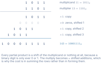
Figure 1 works one example all the way through.
03.Signed Multiplication: Booth’s Algorithm
The shift-and-add algorithm works for unsigned operands. For signed two’s-complement operands, the sign bit must be handled specially. One approach is to convert both operands to positive magnitudes, multiply, and negate the result if the signs disagree. A more elegant approach is Booth’s algorithm, which works directly on signed operands without conversion.
The basic idea
Booth’s insight starts from a simple identity about runs of consecutive 1-bits. Consider the binary number . The run of three 1-bits at positions 3, 2, 1 can be replaced by a subtraction and an addition:
Instead of three additions (one per 1-bit), the multiplier performs one addition (at the position one above the run’s MSB) and one subtraction (at the run’s LSB). For long runs of 1-bits this dramatically reduces the number of nonzero partial products.
Booth’s algorithm scans the multiplier from right to left, examining pairs of adjacent bits where is an implied zero below the LSB:
Table 2. Booth recoding rules. The action is determined by the pair (B[i], B[i-1]).
| Action | ||
|---|---|---|
| 0 | 0 | No operation (middle of a run of 0s) |
| 0 | 1 | Add (end of a run of 1s) |
| 1 | 0 | Subtract (beginning of a run of 1s) |
| 1 | 1 | No operation (middle of a run of 1s) |
Because the algorithm uses subtraction as well as addition, the partial products are signed. The partial product register must be treated as a signed two’s-complement value throughout, and the arithmetic right shift (which preserves the sign bit) replaces the logical right shift of the unsigned algorithm.
Radix-4 Booth recoding
Basic Booth’s algorithm examines one multiplier bit per cycle and still takes cycles. The practical speedup comes from radix-4 Booth recoding (also called modified Booth encoding), which examines two bits at a time and halves the number of partial products from to .
The recoding groups the multiplier bits into overlapping 3-bit windows: for , with . Each window selects one of five operations on the multiplicand:
Table 3. Radix-4 Booth recoding. The window (B[2i+1], B[2i], B[2i-1]) determines the partial product contribution for the two-bit group.
| Digit | Partial product | |||
|---|---|---|---|---|
| 0 | 0 | 0 | ||
| 0 | 0 | 1 | ||
| 0 | 1 | 0 | ||
| 0 | 1 | 1 | ||
| 1 | 0 | 0 | ||
| 1 | 0 | 1 | ||
| 1 | 1 | 0 | ||
| 1 | 1 | 1 |
The five distinct operations are , , and . The values are obtained by shifting left by one position, which costs no hardware. The negation is the bitwise complement plus one, which can be folded into the carry-save addition. Every production integer and floating-point multiplier uses radix-4 Booth recoding to halve the partial product count before feeding the results into a tree reduction network.
04.Fast Multipliers: Tree Reduction
Even with radix-4 Booth recoding, a 64-bit multiply still generates 32 partial products. Adding them sequentially would take 31 addition steps, each with a carry chain delay. The key to a single-cycle multiplier is to add the partial products in parallel using a tree of carry-save adders (CSAs).
The carry-save adder
A carry-save adder is a row of independent full-adders with no carry chain connecting them. Three -bit inputs (, , ) produce two -bit outputs: a sum vector and a carry vector , where bit of and are the sum and carry outputs of a single full-adder operating on . Because there is no carry propagation, the entire operation completes in a single full-adder delay (two gate levels).
The three-input sum is not lost. It is preserved in redundant form: (the factor of two arises because each carry bit represents a value one position to the left). A CSA therefore reduces three numbers to two numbers without any carry propagation. Repeating this reduction in a tree structure reduces partial products to two final vectors in stages.
Wallace trees
A Wallace tree reduces partial products to two numbers (a sum vector and a carry vector) in the minimum number of CSA stages. The algorithm is greedy: at each stage, group as many numbers as possible into sets of three, reduce each set to two via a CSA, and pass any leftover numbers (one or two that do not form a complete group of three) unchanged to the next stage.
The number of CSA stages for partial products is . For a 64-bit unsigned multiply ( partial products), that is stages. With radix-4 Booth recoding ( partial products), the count drops to stages.
After the tree reduction produces two final vectors, a single carry-propagate adder (CPA), typically a fast prefix-tree adder from Chapter 5, adds them to produce the -bit product. The total multiplier delay is therefore:
where is the Booth recoding delay (one mux level), is one carry-save stage delay (one full-adder), and is the final carry-propagate adder delay ( for a prefix-tree adder).
Dadda trees
A Dadda tree is a variant of the Wallace tree that uses the same reduction stages but delays reductions as long as possible. Where the Wallace tree eagerly reduces every column to the minimum height at each stage, the Dadda tree reduces each column only to a target height determined by the sequence working backward from (the final two rows). The first few target heights are .
The Dadda tree produces the same number of stages as the Wallace tree for any given number of partial products, but it uses fewer full-adder and half-adder cells overall because it does not perform reductions that are not yet necessary. The tradeoff is that intermediate columns can be taller, which increases wire length in the physical layout. In practice, modern multiplier designs blend aspects of both approaches, choosing the reduction pattern that minimizes the product of delay and area for the target process technology.
The final adder
The tree reduction produces two -bit numbers. The final step is a single carry-propagate addition to produce the -bit product. This adder is on the critical path, so it uses the fastest adder topology available: typically a Kogge-Stone or Han-Carlson prefix adder (a later section in Chapter 5). The final adder accounts for a significant fraction of the total multiplier delay, so some designs use a custom hybrid adder that is optimized for the specific bit pattern of the tree’s output.
05.Division: Restoring and Non-Restoring
Division is the inverse of multiplication. Given a dividend and a divisor , the division computes a quotient and a remainder such that with . Division is intrinsically sequential: each quotient bit depends on the sign of the partial remainder after subtracting the divisor, and that sign is not known until the subtraction completes. There is no division equivalent of the Wallace tree that computes all quotient bits in parallel.
Restoring division
The restoring division algorithm mirrors the pencil-and-paper long division process.
The restore step is the algorithm’s weakness. In the worst case, every iteration requires both a subtraction and a restoration addition, doubling the number of adder operations compared to multiplication.
Non-restoring division
The non-restoring division algorithm eliminates the restore step. The key observation is that restoring by adding and then shifting left is equivalent to shifting the negative partial remainder left and adding on the next iteration (because the restoring path computes on the next step, which is exactly the value that shifting the negative remainder and adding produces).
The rule becomes:
-
Shift left by one position.
-
If , subtract . If , add .
-
Set if the new is non-negative, and set otherwise.
Each iteration uses exactly one adder operation (either add or subtract), cutting the worst-case cycle count in half compared to restoring division. Conceptually the algorithm produces quotient digits from the redundant set , one per iteration, which the hardware records as the bits 1 and 0, and the result may require a final correction step if the last partial remainder is negative.
06.SRT Division
SRT division (named for Sweeney, Robertson, and Tocher, who independently described the method in 1958) is a higher-radix extension of non-restoring division. Where non-restoring division produces one quotient bit per iteration, a radix- SRT divider produces quotient bits per iteration.
The key idea is to use a redundant quotient digit set. A radix-4 SRT divider selects each quotient digit from the set instead of the minimal set . The redundancy means that the quotient digit can be selected from an approximate inspection of the top few bits of the partial remainder and the divisor, using a small lookup table called the quotient selection table (QST). The approximation avoids the need for a full-precision comparison, which would otherwise be on the critical path.
The radix-4 SRT division step is:
-
Shift the partial remainder left by 2 positions (multiply by 4).
-
Look up the quotient digit in the QST based on the top several bits of the shifted partial remainder and the divisor.
-
Update the partial remainder: .
Each iteration retires 2 quotient bits. A 53-bit floating-point mantissa division for IEEE 754 double precision, where the significand is 52 stored fraction bits plus an implicit leading one, requires 27 iterations of a radix-4 SRT divider, compared to 53 iterations for a non-restoring divider. At one iteration per cycle, SRT roughly halves the division latency.
07.Division by Convergence: Newton-Raphson
A fundamentally different approach to division avoids the sequential quotient-bit-by-bit process entirely. The Newton-Raphson method computes by iterating a recurrence that doubles the number of correct bits with each step. Once is known, the quotient is obtained by a single multiplication .
The recurrence is:
Starting from an initial approximation (obtained from a lookup table indexed by the top bits of ), each iteration squares the relative error: if has correct bits, then has correct bits. For a 53-bit mantissa, starting from a 10-bit table lookup requires only three iterations ( bits) to converge.
Each iteration requires two multiplications and one subtraction (or equivalently, two fused multiply-add operations). If the processor already has a fast pipelined multiplier, Newton-Raphson can produce a quotient in fewer cycles than SRT division, especially when the multiplier has a throughput of one multiplication per cycle. The AMD K5 and IBM POWER series are examples of processors that have used Newton-Raphson for floating-point division.
The disadvantage is that Newton-Raphson produces a rounded approximation to , not an exact quotient and remainder. For integer division (which requires an exact remainder), an additional multiply-subtract step is needed to compute and to correct if or .
08.Modular Arithmetic
Modular arithmetic is arithmetic performed with respect to an integer modulus . The result of every operation is reduced to the range . Modular addition, subtraction, and multiplication follow the rules:
\begin{align} (a + b) \bmod m &= ((a \bmod m) + (b \bmod m)) \bmod m \\ (a - b) \bmod m &= ((a \bmod m) - (b \bmod m) + m) \bmod m \\ (a \times b) \bmod m &= ((a \bmod m) \times (b \bmod m)) \bmod m \end{align}
These identities allow each intermediate result to be reduced modulo before the next operation, keeping the operand width bounded.
Hardware reduction
When is a power of two, reduction is free: the result is simply the low bits of the full-precision output, which is a bit mask or a truncation. This is why address arithmetic in a processor with a -entry cache uses the low bits of the address as the cache index.
When is not a power of two, reduction requires a division (or a multiplication by the modular inverse, if is known at design time). Barrett reduction and Montgomery reduction are two well-known techniques that replace the division with a sequence of multiplications and shifts, and they are central to cryptographic arithmetic, which lies beyond this book.
Applications in processor design
Modular arithmetic appears throughout a processor:
-
CRC computation. Cyclic redundancy checks used in networking and storage are polynomial divisions in , implemented as LFSR-based modular reduction circuits.
-
Address hashing. Cache set indexing, branch predictor indexing, and TLB lookup all use modular arithmetic (often a simple power-of-two mask) to map large address spaces into small tables.
-
Wrap-around counters. Program counters, sequence numbers, and circular buffer pointers use modular increment.
-
Cryptographic accelerators. AES, SHA, RSA, and the post-quantum lattice-based schemes all require modular multiplication or modular exponentiation as a core operation.
09.Looking Ahead
This chapter has built the integer multiplier and divider that sit inside the execution unit of every general-purpose CPU. The shift-and-add baseline gave way to Booth recoding for signed operands, Wallace and Dadda trees for parallel partial-product reduction, SRT for fast multi-bit division, and Newton-Raphson for division through convergence. The next chapter extends the arithmetic story to floating-point numbers, where the same multiplier and divider hardware is reused with different exponent and mantissa handling on top.
10.Worked Examples
11.Exercises
References
- [1]Patterson, David A. and Hennessy, John L. (2020). “Computer Organization and Design RISC-V Edition: The Hardware Software Interface.” Morgan Kaufmann.