Introduction to Pipelining
September 13, 202628 min readintermediate
The multi-cycle CPU of Chapter 27 reduces the clock period by splitting each instruction into phases. It cannot, however, reduce the cycles-per-instruction count. R-type arithmetic still takes four cycles. A…
The multi-cycle CPU of Chapter 27 reduces the clock period by splitting each instruction into phases. It cannot, however, reduce the cycles-per-instruction count. R-type arithmetic still takes four cycles. A load takes five. The pipelined design described in this chapter takes the next step. It keeps the short clock period but overlaps the execution of successive instructions so that, in steady state, one instruction completes every cycle.
The intuition is captured by an analogy first popularized by David Patterson: doing laundry. A single load of laundry goes through four stages: washing, drying, folding, and putting away. Each stage takes 30 minutes. To do four loads sequentially takes minutes. But the four stages use separate equipment (the washer, the dryer, the table, and the closet). After the first load finishes washing, it can move to the dryer while the second load starts washing. After the second load finishes washing, it can move to the dryer while the third load starts washing, and the first load (already dry) moves to folding. After about 30 minutes per stage transition, all four loads are in different stages simultaneously. The total time drops to minutes. The savings come from running stages in parallel, not from making any stage faster.
This chapter develops the same idea for an RV32I CPU. The five instruction phases identified in Chapter 27 (IF, ID, EX, MEM, WB) become five pipeline stages. The pipeline registers between stages hold the per-instruction state that flows downstream. The chapter computes ideal pipeline speedup, identifies the five ideal assumptions, and shows where each breaks in practice. The stage-by-stage design of the datapath belongs to Chapter 29, the detailed treatment of hazards (forwarding, stalling, squashing) to Chapter 30, and exceptions and interrupts to Chapter 31.
01.The Laundry Analogy in Detail
The laundry analogy deserves careful unpacking before the hardware version is drawn. The structure of the analogy maps exactly onto pipeline arithmetic.
Four loads, four stages, 30 minutes each
Consider four loads of laundry called , , , , each requiring 30 minutes of washing, 30 minutes of drying, 30 minutes of folding, and 30 minutes of putting away. The four stages use four distinct pieces of equipment.
Sequential execution
If only one load is in progress at a time, the schedule is:
Table 1. Sequential schedule of four laundry loads. Time in 30-minute intervals.
| Slot | 1 | 2 | 3 | 4 | 5 | 6 | 7 | 8 | 9 | 10 | 11 | 12 | 13 | 14 | 15 | 16 |
|---|---|---|---|---|---|---|---|---|---|---|---|---|---|---|---|---|
| W | D | F | P | |||||||||||||
| W | D | F | P | |||||||||||||
| W | D | F | P | |||||||||||||
| W | D | F | P |
W = washing, D = drying, F = folding, P = putting away. Total time = 16 slots = 8 hours.
Pipelined execution
If a load moves to the next stage as soon as it finishes the previous, and the next load starts as soon as the previous load vacates the washer, the schedule becomes:
Table 2. Pipelined schedule of four laundry loads.
| Slot | 1 | 2 | 3 | 4 | 5 | 6 | 7 |
|---|---|---|---|---|---|---|---|
| W | D | F | P | ||||
| W | D | F | P | ||||
| W | D | F | P | ||||
| W | D | F | P |
Total time = 7 slots = 3.5 hours. The pipelined schedule is faster than the sequential schedule for four loads. For a much longer sequence (say loads), the total time approaches slots, against the sequential slots, for a speedup of as grows without bound. Four stages, fourfold speedup in the limit.
What the analogy teaches
Three lessons carry over to CPU pipelining unchanged. First, each load (instruction) still spends 4 slots (cycles) from start to finish. Latency is unchanged. Second, the throughput improves from 1 load per 4 slots to 1 load per slot in steady state. That is the pipeline speedup. Third, the schedule is not full immediately. During the first three slots the pipeline is still filling and fewer than four loads are in flight, and during the last three slots it is draining. The pipeline takes some startup (fill) and some shutdown (drain) time. For four loads the fill plus drain (3 + 3 = 6 slots of partial utilization) eats into the asymptotic 4x speedup.
02.The Five-Stage RV32I Pipeline
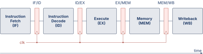
The classical RISC pipeline, introduced with the Berkeley RISC I and the Stanford MIPS in the early 1980s, has five stages. They correspond directly to the five phases identified in the multi-cycle design.
Stage names and activities
IF (Instruction Fetch). Read the instruction word at the address in the PC. Update the PC to PC + 4.
ID (Instruction Decode and register read). Decode the instruction. Read the source registers from the register file. Sign-extend the immediate.
EX (Execute). Perform the ALU operation. For arithmetic, compute the result. For loads and stores, compute the effective address. For branches, compute the comparison and the target.
MEM (Memory access). Read or write data memory. Arithmetic instructions do nothing in this stage but still take one cycle.
WB (Writeback). Write the result (from EX or MEM) back to the register file.
Each stage takes one clock cycle. The clock period is set by the slowest single stage. The dominant blocks in the single-cycle timing model of the table below are the memory access (about 2.0 ns) and the ALU (about 2.0 ns), and dividing that model’s 9.1 ns worst-case path into five roughly balanced stages leaves about 1.8 ns of logic in the slowest stage. Adding the pipeline register’s clock-to-Q and setup margin (about 0.2 ns per stage) gives ns, the value used throughout this chapter.
The pipelined datapath
Pipeline registers carry per-instruction state
The pipeline registers between stages carry every piece of information that the downstream stages will need about the instruction currently in flight. The contents of each register expand from left to right because each stage adds new values:
IF/ID: instruction word (32 bits), PC (32 bits). Total 64 bits.
ID/EX: register file read data (rs1 value, rs2 value = 2 32 bits), immediate (32 bits), PC (32 bits), rd field (5 bits), control signals (about 10 bits). Total bits.
EX/MEM: ALU result (32 bits), B (rs2 value, for SW) (32 bits), rd field (5 bits), control signals for MEM and WB stages (about 6 bits). Total bits.
MEM/WB: ALU result (32 bits, for non-load), memory read data (32 bits, for load), rd field (5 bits), control signals for WB stage (about 3 bits). Total bits.
The total pipeline register storage is on the order of 350 bits, or about 40 bytes. This is a small but nonzero hardware cost relative to the architectural register file (32 registers 32 bits = 1024 bits = 128 bytes).
03.Ideal Speedup Analysis
What speedup can a pipelined CPU achieve compared with the single-cycle CPU it replaced?
The fundamental formula
If the pipeline has stages, each stage takes time , and the single-cycle equivalent takes time (one cycle of the full datapath), then for instructions:
-
Single-cycle total time = .
-
Pipelined total time = .
The extra cycles in the pipelined total are the fill overhead: it takes cycles after the first instruction enters IF before the first instruction exits WB and the pipeline is fully populated.
Pipeline speedup formula
The ratio of single-cycle to pipelined execution time is:
where the second equality uses .
For large , the formula approaches , the number of stages. A 5-stage pipeline approaches speedup in the limit.
Speedup at finite N
For small programs, the fill overhead matters.
Table 3. Speedup of a 5-stage pipeline over the single-cycle CPU at different N.
| instructions | Speedup |
|---|---|
| 1 | |
| 2 | |
| 5 | |
| 10 | |
| 100 | |
| 1000 | |
| 5.0 |
For programs of even modest length (100 instructions or more), the asymptotic speedup is closely approached. Real programs execute billions of instructions, so the fill overhead is negligible.
04.Why Real Speedup Falls Short of k
The ideal speedup formula assumes that one instruction enters and one exits the pipeline every cycle. Real pipelines fail to achieve this for three reasons, collectively called pipeline hazards.
Structural hazards
A structural hazard occurs when two instructions in different stages need the same hardware resource in the same cycle. The multi-cycle design’s unified memory is a structural hazard if ported directly into a 5-stage pipeline. In cycle , the instruction in IF stage wants to read the memory for instruction fetch. The instruction in MEM stage (three stages downstream) wants to access memory for a load or store. Both require the memory port simultaneously. With one port, one of them must wait, stalling the pipeline.
The remedy is to provide two memory ports, typically realized by splitting into separate instruction and data caches. The 5-stage RISC pipeline of MIPS and ARM has this split from the start.
Data hazards
A data hazard occurs when an instruction needs the result of an earlier instruction that has not yet finished. Consider:
A data hazard between two instructions
| add x3, x1, x2 ; produces x3 | |
| sub x4, x3, x5 ; reads x3 |
The ADD produces x3 in cycle 5 (its WB stage). The SUB reads x3 in cycle 3 (its ID stage if it follows the ADD immediately). The data is not yet in the register file when the SUB tries to read it. Without intervention, the SUB reads a stale value.
Three remedies exist, each treated in detail in Chapter 30.
-
Forwarding (bypassing): route the ALU output of the
ADD(available at end of cycle 3 in EX) directly into the EX stage input of theSUB(needed at start of cycle 4). The result skips the register file write and read. -
Stalling: hold the
SUBin the ID stage for two extra cycles until theADD’s WB completes. The pipeline runs slower by exactly two cycles. -
Compiler reordering: place unrelated instructions between the producer and consumer. This works only if the compiler finds such instructions.
Real pipelines combine forwarding (which is free in cycles, only costs wires) with stalling for load-use hazards that forwarding cannot resolve.
Control hazards
A control hazard occurs at branches. The IF stage of cycle fetches an instruction at PC. If the previous instruction was a branch that ends up taken, the new PC is not the sequential PC+4 but the branch target. The branch decision is computed in EX (cycle 3 of the branch’s lifetime), which is two cycles after its IF. The IF stages of cycles 2 and 3 have already fetched instructions assuming the branch is not taken. If the branch is in fact taken, those fetches are wrong and must be squashed.
The cost of squashing two instructions is two stall cycles. With 20% of instructions being branches and half of them taken, the average control-hazard penalty is cycles per instruction. This brings the effective CPI from 1.0 to 1.2 and the speedup from 5x to about 4.2x.
Branch prediction, previewed in Chapter 30 and treated in detail in another chapter, reduces the penalty by guessing the branch outcome at fetch time. A well-predicted branch costs zero stall cycles. A mispredicted branch costs the full pipeline depth in flush cycles.
05.The Five Ideal Assumptions
The ideal pipeline speedup of rests on five assumptions, each violated in real CPUs.
Assumption 1: Every stage takes exactly one cycle
The ideal assumes every stage’s combinational delay is the same. Real stages differ. The MEM stage in particular is variable: a cache hit is one cycle, a cache miss is hundreds of cycles. The clock period must accommodate the slowest stage. Variable-latency stages stall the pipeline. Cache hierarchies, the subject of Part IV, are partly motivated by the need to keep MEM-stage latency under control.
Assumption 2: One instruction enters per cycle
The ideal assumes the IF stage always fetches a new instruction. A branch misprediction can cause the IF stage to fetch wrong instructions. A long-latency stall (cache miss in IF, exception) can leave the IF stage idle. Both reduce the effective fetch rate below 1.0.
Assumption 3: All stages are independent
The ideal assumes that the work in stage at cycle does not depend on the work in stage at the same cycle. Data hazards violate this assumption directly. Forwarding resolves most cases, but load-use hazards still require at least one stall cycle.
Assumption 4: No structural conflicts
The ideal assumes any pair of stages can run concurrently without contending for shared hardware. The textbook 5-stage RISC pipeline achieves this by splitting the memory port (IF and MEM use separate caches) and using separate read and write ports on the register file. CISC instructions sometimes need more than one ALU operation or more than one memory access per instruction, creating structural conflicts that require pipeline duplication or stalls.
Assumption 5: No exceptions or interrupts
The ideal assumes the program executes straight through without interruption. Exceptions (illegal instructions, page faults, divide by zero) and interrupts (external device requests, timer expirations) force the pipeline to flush in-flight instructions and jump to a handler. Precise exception handling (restoring the architectural state to exactly the point of the faulting instruction) is the subject of Chapter 31, and it returns with the reorder buffer in Part V.
The realized speedup in practice
For a well-designed RISC pipeline with branch prediction, forwarding, and split caches, the CPI in steady state is typically 1.1 to 1.3 for integer code on a 5-stage pipeline. The realized speedup over the equivalent single-cycle design is about . For load-heavy or branch-heavy code, the CPI grows and the speedup shrinks. For a deeper in-order pipeline of 10 to 15 stages, still issuing one instruction per cycle, the CPI may grow to 1.5 or 2.0, but the clock frequency rises in compensation.
06.The Throughput-Latency Distinction
A central conceptual point: pipelining improves throughput, not latency.
Throughput
The pipelined CPU completes one instruction per cycle in steady state. With ns, that is 500 million instructions per second. The single-cycle CPU at ns completes one instruction per 9 ns, or 111 million instructions per second. The pipelined CPU has higher throughput.
Latency
A single instruction still takes 5 cycles to traverse the pipeline. In the pipelined CPU, that is ns of latency. In the single-cycle CPU, the same instruction takes 9 ns. The latency of a single instruction is actually 11% worse in the pipelined design, because of the pipeline-register overhead between stages.
If the program is purely sequential and contains a single dependency chain (each instruction depends on the previous), the pipeline cannot hide the dependence and the CPI rises above 1. With no forwarding at all, each consumer waits two extra cycles in ID for its producer’s writeback, which is one new instruction every three cycles rather than one per cycle. Forwarding recovers most of that, but a chain of loads and their immediate uses still costs one stall cycle per pair. This is the floor on what pipelining can achieve.
Why throughput matters more
Most programs have many independent instructions. A modern compiler arranges code so that there are several cycles’ worth of unrelated work between any two dependent instructions. The pipeline benefits from this independence by overlapping. The total execution time is dominated by throughput, not by the latency of any individual instruction.
For latency-bound code (such as a tight pointer-chasing loop through a linked list), throughput-oriented pipelining offers no help. The CPU is constrained by the memory latency of each pointer dereference. Latency-bound workloads motivate the cache hierarchy treated in Part IV.
07.The Pipeline Diagram
Throughout the next several chapters, the standard way to visualize pipeline behavior is the pipeline diagram. It plots instructions on the vertical axis and cycles on the horizontal axis, with each cell labeled by the stage in which the instruction is executing during that cycle.
Example: four instructions, no hazards
Table 4. Pipeline diagram for four instructions with no hazards.
| Cycle | 1 | 2 | 3 | 4 | 5 | 6 | 7 | 8 |
|---|---|---|---|---|---|---|---|---|
ADD x3, x1, x2 | IF | ID | EX | MEM | WB | |||
SUB x6, x4, x5 | IF | ID | EX | MEM | WB | |||
AND x9, x7, x8 | IF | ID | EX | MEM | WB | |||
OR x12, x10, x11 | IF | ID | EX | MEM | WB |
In cycle 5, five instructions are in flight simultaneously: the ADD is in WB, the SUB is in MEM, the AND is in EX, the OR is in ID, and the next instruction (not shown) is in IF. Five stages, five instructions in flight. The pipeline is full.
Example: a data hazard with one stall
Table 5. Pipeline diagram with a load-use hazard requiring a one-cycle stall.
| Cycle | 1 | 2 | 3 | 4 | 5 | 6 | 7 | 8 |
|---|---|---|---|---|---|---|---|---|
LW x3, 0(x1) | IF | ID | EX | MEM | WB | |||
ADD x4, x3, x5 | IF | ID | - | EX | MEM | WB | ||
SUB x6, x4, x7 | IF | - | ID | EX | MEM | WB |
The ADD consumes x3 produced by the LW. The LW produces x3 at the end of its MEM stage (cycle 4), too late for the ADD’s EX stage at the start of cycle 4. The pipeline stalls one cycle (shown as ), inserts a bubble, and the ADD then proceeds in cycle 5. The downstream SUB is also delayed by one cycle.
Example: a control hazard from a taken branch
Table 6. Pipeline diagram showing a taken branch flushing two instructions.
| Cycle | 1 | 2 | 3 | 4 | 5 | 6 | 7 | 8 |
|---|---|---|---|---|---|---|---|---|
BEQ x1, x2, target | IF | ID | EX | MEM | WB | |||
(seq instr 1) | IF | ID | - | - | ||||
(seq instr 2) | IF | - | - | |||||
(target instr) | IF | ID | EX | MEM | WB |
The BEQ executes in EX during cycle 3 and decides the branch is taken. The two sequential instructions that were fetched in cycles 2 and 3 must be squashed. The instruction at the branch target is fetched starting in cycle 4. Two cycles are lost.
These three patterns (clean execution, data hazard with stall, control hazard with flush) are the building blocks of every pipeline analysis in subsequent chapters.
08.Pipeline Implementation Sketch
A complete RV32I 5-stage pipeline implementation is large enough to be the subject of an entire course project. Chapter 34 walks through the project. This section sketches just enough of the implementation to motivate the deeper treatment of hazards in Chapter 30.
The pipeline registers in SystemVerilog
Pipeline register skeleton
// IF/ID pipeline register
typedef struct packed {
    logic [31:0] pc;
    logic [31:0] instruction;
} if_id_t;

if_id_t if_id_reg;

always_ff @(posedge clk) begin
    if (reset || flush) begin
        if_id_reg <= '0;
    end else if (!stall) begin
        if_id_reg.pc          <= pc;
        if_id_reg.instruction <= imem_data;
    end
end
The structure repeats for each pipeline register (IF/ID, ID/EX, EX/MEM, MEM/WB), with increasing payload at each successive register. The flush signal clears the register (for control hazards). The stall signal holds the value (for data hazards). Both signals come from a hazard-detection unit that is the subject of Chapter 30.
The hazard detection unit
A small combinational block inspects the pipeline registers and detects when the next instruction’s source registers match the destination register of an instruction currently in EX or MEM (or WB, depending on the forwarding strategy). When a hazard is detected, the block asserts stall for the IF and ID stages, and flush for any squashed stages.
The forwarding unit
A small combinational block inspects the pipeline registers and, when an EX-stage instruction needs a value that is being produced by the EX or MEM stage of an earlier instruction, routes the value directly through a multiplexer at the ALU’s operand inputs. This is the same wire-only technique used in Chapter 25 to send the ALU output back to the register file’s write port, applied here across pipeline stages.
What is not yet shown
The full implementation requires the hazard detection unit, the forwarding unit, the branch prediction unit (or a stall-on-branch policy), the precise exception handling logic, and the I-cache and D-cache interfaces. Each of these is a chapter in itself. The pipeline introduced here is the chassis. Subsequent chapters add the suspension, brakes, and steering.
09.A Historical Note
Pipelining as a CPU organization technique dates to the 1960s. The IBM 7030 Stretch (1961) was the first commercial CPU with a multi-stage pipeline. The CDC 6600 (1964), designed by Seymour Cray, used a four-stage pipeline for its central processor and ten functional units for parallel execution. The IBM System/360 Model 91 (1967) implemented Tomasulo’s algorithm for dynamic instruction scheduling in a pipelined processor, the ancestor of every modern out-of-order CPU.
Pipelining did not become standard in commodity microprocessors until the 1980s, when the RISC movement made fixed-length, regular instructions practical to pipeline in a few hundred thousand transistors. The MIPS R2000 (1985) had a 5-stage pipeline almost identical to the textbook diagram above. The SPARC V7 (1987), the ARM ARM2 (1986, three-stage), and the DEC Alpha 21064 (1992) all built on the same template.
Intel’s 80486 (1989) was the first pipelined x86 CPU, with a five-stage integer pipeline. The Pentium (1993) was the first superscalar x86, using a dual-pipeline organization that issued two instructions per cycle. The Pentium Pro (1995) added out-of-order execution on top of the pipeline. By 2000, every commercial high- performance CPU was pipelined.