Time is the loop counter. Every module gets asked "what do you do this cycle?" every single cycle. This is a cycle-driven or time-stepped simulator and it is exactly right for something like a CPU pipeline, where every stage genuinely has work every cycle.
Now point it at a memory controller. A DRAM bank in an open-page policy might do something meaningful once every forty cycles: activate a row, wait, read a column, wait, precharge. In between there is nothing. The loop still calls bank->tick() forty times, thirty-nine of which are a function call that immediately returns after checking a counter.
Put a number on it. Sixteen banks, a hundred million simulated cycles, one meaningful action per bank per forty cycles. Useful work is 16×108/40=4×107 actions. Calls made are 16×108=1.6×10⁹. You performed forty times more calls than actions, and the ratio gets worse as the model gets more detailed and the structures get slower.
The fix is to stop asking and start being told. Instead of polling every module every cycle, let a module say "wake me at cycle 40 and not before." That is discrete-event simulation, and it is the technique SiFive names by title.
Do this on paper first. It is small enough to fit on one page and once you have traced it, the code in 2.3 is obvious rather than mysterious.
The system. A requester issues memory requests, one every three ticks, three requests total, and it does not wait for a response before issuing the next one. Each request goes somewhere with a different latency: request 0 takes 10 ticks, request 1 takes 4 ticks, request 2 takes 5 ticks. Nothing else happens.
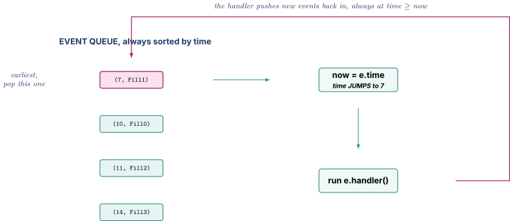
The state. There is exactly one piece of machinery: a list of things that are going to happen, each stamped with the tick at which it happens. Call it the event queue. It is always kept sorted by timestamp, earliest first. There is also one variable, now, holding the current simulated time.
The rule. Repeat: take the earliest event out of the queue, set now to that event's timestamp, run the event, and let the event put new events into the queue. Stop when the queue is empty.
Trace it.
Step
Queue before
Pop
now becomes
What the handler does
Queue after
init
n/a
n/a
0
seed the first issue
(0,Issue0)
1
(0,I0)
(0,I0)
0
send request 0, latency 10, so schedule Fill0 at 0+10, and also schedule Issue1 at 0+3
(3,I1),(10,F0)
2
(3,I1),(10,F0)
(3,I1)
3
send request 1, latency 4, schedule F1 at 3+4=7, and schedule I2 at 3+3=6
(6,I2),(7,F1),(10,F0)
3
(6,I2),(7,F1),(10,F0)
(6,I2)
6
send request 2, latency 5, schedule F2 at 6+5=11, and no more issues
(7,F1),(10,F0),(11,F2)
4
(7,F1),(10,F0),(11,F2)
(7,F1)
7
request 1 completes
(10,F0),(11,F2)
5
(10,F0),(11,F2)
(10,F0)
10
request 0 completes
(11,F2)
6
(11,F2)
(11,F2)
11
request 2 completes
empty, stop
Six things to take from that table, and every one of them is a real property of the technique rather than an accident of this example.
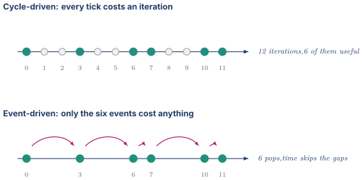
Time jumped.now went 0, 3, 6, 7, 10, 11. It never took the values 1, 2, 4, 5, 8, 9 because nothing happened at those ticks and there was nothing to compute. A cycle-driven loop would have executed twelve iterations. This did six. The cost of a discrete-event simulation is proportional to the number of events, not to the length of simulated time. That single sentence is most of the answer to "why discrete-event."
Completion order fell out for free. Requests completed in the order 1, 0, 2, which is not the order they were issued. Nobody wrote any code to reorder anything. Out-of-order completion is what a sorted-by-time queue does automatically, which is why this structure models non-blocking behaviour so naturally.
The future is data. At step 3 the queue contained three events with timestamps 7, 10, and 11. Those are commitments already made. The simulator's entire knowledge of the future lives in that one container.
Handlers only schedule forward. Every event scheduled a new event at a time strictly greater than or equal to now. If a handler ever schedules something in the past, the simulation has violated causality, and there is no sensible recovery. Assert on it.
The queue is the only global. No module talks to the clock. Modules talk to the queue.
Termination is a queue property. The run ended because the queue drained. Real simulators also stop at a horizon, or when a workload signals completion, but "no more events" is the natural end.
using Tick = uint64_t;struct Event{Tick time;uint32_t priority; // same-time ordering, see 2.4uint64_t seq; // insertion order, the final tiebreakstd::function<void()> handler;};// std::priority_queue is a MAX-heap. We want the EARLIEST time first,// so the comparator must report "a comes after b", i.e. a is lower// priority than b, when a's timestamp is larger.struct LaterFirst{bool operator()(const Event& a, const Event& b)const{if(a.time != b.time)return a.time > b.time;if(a.priority != b.priority)return a.priority > b.priority;return a.seq > b.seq;}};
The kernel is nine lines.
C++
class Kernel{public:void schedule(Tick when, uint32_t prio, std::function<void()> fn){assert(when >= now_ && "causality violation: scheduled into the past");q_.push(Event{when, prio, nextSeq_++, std::move(fn)});}void run(Tick horizon){while(!q_.empty()&& q_.top().time <= horizon){Event e = q_.top(); // copy outq_.pop(); // then removenow_ = e.time; // time is DATA, not a countere.handler(); // may push more events}}Tick now()const{return now_; }private:std::priority_queue<Event, std::vector<Event>, LaterFirst> q_;Tick now_ = 0;uint64_t nextSeq_ = 0;};
Figure 1. The whole of discrete-event simulation is one sorted container and one loop, where popping the earliest event is what advances time and running that event is what refills the container.
Complexity. A binary heap gives O(logn) for both push and pop where n is the number of events resident in the queue at that moment. If a run processes E events total and the queue never holds more than n, the total cost is O(Elogn). In practice n stays small, in the hundreds or low thousands, because a hardware model only ever has a bounded number of things in flight, so logn is around ten and the heap is not the bottleneck. The bottleneck is almost always inside the handlers.
One implementation note that gets asked. std::function allocates on the heap when the callable it wraps is larger than its small-object buffer, which for a lambda capturing a couple of pointers it usually is not, but for one capturing a fat payload it is. In a hot kernel that per-event allocation is measurable. Production simulators avoid it by making events objects with a virtual process() method that are pre-allocated and reused, which is what gem5 does with its Event class hierarchy. Knowing that trade-off, and being able to say "I'd start with std::function and switch to an intrusive event object if the profiler said so," is a better answer than either choice on its own.
This is where a naive event kernel produces a bug that is genuinely hard to find, so it is worth a concrete example rather than a warning.
A credit-based flow control scheme, of the kind in Interconnect and AMBA, has a counter of available credits. At tick 100 two things happen: a credit is returned by the downstream block, and a credit is consumed by the upstream block. Both were scheduled independently, both landed on tick 100, and the counter currently reads 0.
If consume runs first, the counter goes to −1. If it is an unsigned type it wraps to a very large number and the model now believes it has four billion credits. If it is signed and there is an assertion, the model trips an assertion that describes a condition the hardware never enters.
If return runs first, the counter goes to 1 and then back to 0, and everything is fine.
Which happens? With a plain timestamp-only comparator, it depends on the internal layout of the heap, which depends on what else was inserted and in what order, which depends on the workload. The model is correct on the traces you ran and wrong on the one you did not, and the failure looks like a workload-dependent phantom.
The fix has two halves and you need both. First, priority: give events an explicit priority field so that at a given tick, all credit-return events run before all credit-consume events, by design, stated in the code, matching whatever the RTL actually does. Second, a total order: give every event a monotonically increasing insertion sequence number as the final tiebreak, so that two events with the same tick and the same priority always resolve the same way on every run. Without that, the same binary and the same input can produce different results, and a simulator you cannot reproduce is a simulator you cannot debug.
gem5's Event carries an explicit priority field for exactly this reason, so same-tick ordering there is a stated design decision rather than an accident of the container. I would check the current source for the precise ordering rules among same-tick, same-priority events rather than trust a remembered detail, but the reason the field exists is not in doubt and is the thing worth being able to explain.
The deeper point is the one to say out loud in an interview. The tie-break rule is not an implementation detail, it is part of the model's semantics. It encodes a claim about what the hardware does when two things coincide, and if that claim is wrong, the model is wrong in a way no amount of testing at other timestamps will reveal.
Both approaches are legitimate and the choice is workload-driven, not ideological.
Cycle-driven
Event-driven
Time advances by
one tick per iteration
a jump to the next event
Cost scales with
(cycles) × (modules)
(events) ×log(queue depth)
Wins when
activity is dense, nearly every module every cycle
activity is sparse and bursty
Natural for
a CPU pipeline
DRAM banks, interconnect links, off-chip IO
Code shape
a tick() per module
handlers that reschedule themselves
Ordering discipline
you supply it (Part 5)
the queue supplies part of it, you supply the rest (2.4)
The break-even is easy to reason about. Let A be the fraction of cycles on which a given module actually has work. Cycle-driven costs one call per cycle regardless. Event-driven costs roughly logn heap operations per action, so it costs about Alogn per cycle. Event-driven wins when Alogn<1, which with logn≈10 means it wins when a module is active less than about ten percent of cycles.
That is why real simulators are hybrids. gem5's kernel is event-driven, but an out-of-order CPU model in gem5 essentially schedules itself on every tick, which makes it behave like a cycle-driven model running inside an event-driven kernel, paying the heap cost for no benefit on that one object. Meanwhile the memory system, where activity really is sparse, gets the full benefit. Being able to say "gem5 is event-driven but a busy O3CPU degenerates to cycle-driven, which is why the kernel overhead shows up in profiles of CPU-bound runs" is a considerably better answer than reciting the definition.
For a single-block cache model of the kind in Part 7, driven by a trace, the honest engineering answer is usually cycle-driven, because the block does something almost every cycle and a cycle-driven loop is simpler, faster, and far easier to correlate against RTL because the RTL is also cycle-driven. Say that, and say you know when it stops being the right answer.
Figure 2. The same six actions cost twelve iterations under a cycle-driven loop and six pops under an event-driven kernel, and the gap widens in exact proportion to how idle the modelled block is.
One more thing has to be said now because it recurs in three later parts.
Suppose two events are scheduled at the same tick and one of them produces a value the other consumes. The queue orders them by the tie-break rule of 2.4, so the consumer either sees this tick's value or last tick's value depending on a rule that lives in the kernel rather than in the model. That is fragile, and as the number of same-tick interactions grows it becomes unmanageable.
Hardware solves this with the clock edge. Everything samples the pre-edge value and everything commits after. SystemVerilog encodes that in the non-blocking assignment <=, which you already trust from RTL Design and SystemVerilog. C++ has no <=, so you have to build the equivalent, and that is the two-phase evaluate-then-update discipline of Part 5. SystemC builds it into sc_signal and calls the resulting round trip a delta cycle, which is Part 6.
Three different names, one idea. Notice that now and the later parts will feel like restatements rather than new material.
Performance Modeling lays out the modeling hierarchy and the rule that you use the cheapest model that answers the question. This part goes one level deeper on the three fidelity levels that matter here, because these roles use the words "cycle-accurate" and "performance model" as though they were self-defining, and they are not.
Take one concrete question and answer it three ways. How many outstanding misses per cycle can an L1 sustain with 16 MSHRs and a 200-cycle memory latency? The analytical number below is exact given its assumptions. The two simulated numbers are illustrative figures chosen to show the shape of the divergence rather than measurements from any particular model, and the argument they support does not depend on their exact values.
Analytical. Little's law, from Cache Organization and Prefetching section 7.3. The number in flight equals the arrival rate times the residence time, so N=λL, and rearranging, λ=N/L.
λ=20016=0.08misses per cycle
At 64 bytes a miss and 3 GHz, that is 0.08×64×3×109=15.4 GB/s. Time to produce: about forty seconds with a pen. Assumptions baked in: every MSHR is always usable, memory latency is a constant, there is no queueing anywhere, and the demand stream can always generate another miss.
Cycle-approximate. A few hundred lines of C++. MSHR file modelled as an occupancy counter with a hard limit of 16, memory modelled as a fixed 200-cycle delay with a bandwidth limit, secondary misses merged. Run a trace. It reports 0.078. The 2.5 percent shortfall comes from the tail of the trace where the demand stream runs out of independent misses, which the analytical model had no way to see.
Cycle-accurate. A few thousand lines. The DRAM side now models bank state, row-buffer hits and misses, the timing constraints between activate, read, and precharge, refresh, and the memory controller's scheduling policy. The L1 side models the fill port arbitration and the fact that a fill and a demand access contend for the tag array. It reports 0.061, a 24 percent shortfall against the analytical answer, because on this access pattern most requests are row-buffer misses and the effective latency is far above 200 cycles under load.
Now the point that decides how you spend your life. All three models rank the design options identically. Ask any of them whether 32 MSHRs beats 16, and all three say yes and all three say the improvement is sublinear. The analytical model is off by 24 percent in absolute terms and is completely correct about the decision you were trying to make.
That is the discipline. Know what question you are answering. Absolute throughput for a datasheet needs the cycle-accurate model. Choosing between 8, 16, and 32 MSHRs does not.
The row people forget is maintenance. A cycle-accurate model is a claim about a specific RTL implementation. Every time that RTL changes (a pipeline stage added for timing closure, an arbitration policy changed, a bypass removed to save area), the model becomes wrong, and it becomes wrong silently, because it still runs and still produces plausible numbers. A cycle-accurate model that has not been re-correlated in six months is not a cycle-accurate model, it is a historical document. That is a genuinely senior observation and it is cheap to say.
The cost that people also forget in the other direction is that an analytical model is not free of risk either. It is free of maintenance risk but it fails in the specific way Performance Modeling section 2.2 describes, which is that it has no representation of interaction at all. The moment a queue fills or two mechanisms contend, the equation is not approximately right, it is structurally unable to be right.
Nobody's cycle-accurate model is bit-and-cycle identical to the RTL for all possible inputs. If it were, it would be the RTL, and it would run at the RTL's speed, and there would be no reason to have it.
What the term means in practice, in every organisation, is roughly this. The model reproduces the RTL's cycle count on the correlation suite to within a stated tolerance, and the divergences that remain are documented, understood, and bounded.
Every clause in that sentence is load-bearing.
On the correlation suite means not on all inputs. The model's accuracy claim is scoped to the stimulus it was validated against, exactly like a coverage claim in Verification Methodology.
To within a stated tolerance means a number, typically one to three percent, and you must say whether that is a mean, a mean absolute percentage error, or a worst case, because those are three different numbers and quoting the friendliest one without saying which is the kind of thing that gets caught.
Documented, understood, and bounded means a list, with magnitudes, of the places the model knowingly differs.
Say this in an interview and it does two things at once. It shows you know the term is a claim rather than a category, and it sets you up to talk about the correlation study of Part 8, which is where you actually want the conversation to go.
There is one more distinction worth having ready because it separates people who have built these from people who have used them. Cycle-accurate is not the same as timing-accurate. A cycle-accurate model says a cache access takes four cycles. It says nothing at all about whether four cycles' worth of logic fits in the clock period, whether the tag comparators close timing at eight ways, or whether the array's sense amplifiers settle in time. Those are the questions STA Synthesis and Physical Design and SRAM Arrays and ECC answer, and the model is structurally blind to them. A model that says "16 ways is fine" is saying something about hit rate and nothing whatsoever about whether 16 ways is buildable. Naming that blindness unprompted is a strong move, and it is a place where your background is genuinely ahead of a pure-software modeller's.
Start analytical always, because it costs forty seconds and it kills bad ideas outright, as the AMAT example in Performance Modeling section 2.2 shows. Escalate to cycle-approximate the moment two mechanisms interact or a queue can fill, which in practice is almost immediately for anything with backpressure. Escalate to cycle-accurate only when the question genuinely requires absolute cycle counts, which means correlation against RTL, or a contractual latency number, or a decision where two options are within a few percent of each other and the few percent matters. Escalating too early costs months. Escalating too late produces a confident wrong answer. That is the same rule as Performance Modeling section 2.7, and it is worth being able to state without hedging.
That works and it is what a great deal of production C looks like. Its weaknesses are that nothing stops a caller from reaching into c->tags directly, nothing forces cache_free to be called, and the fact that these three functions belong together is a convention held together by naming.
The C++ version says the same thing with the relationship made explicit.
C++
class Cache{
public:
Cache(int sets, int ways); // constructor: build a valid object
bool lookup(uint64_t addr); // member function
void insert(uint64_t addr);
private:
std::vector<uint32_t> tags_; // owns its storage
int sets_;
int ways_;
};
At the machine level almost nothing changed. c.lookup(addr) compiles to the same thing as cache_lookup(&c, addr). The object's address is passed as a hidden first argument, available inside the function as this. That is the entire mechanism. A member function is a free function with an implicit pointer parameter.
Three things did change and each is worth a sentence.
private is a compile-time check with zero runtime cost. The compiler refuses to compile code outside the class that touches tags_. The generated machine code is identical to the C version. You pay nothing and you get the guarantee that if tags_ is corrupted, the bug is inside this class, which on a 3000-line model is the difference between a ten-minute debug and a two-day one.
The constructor guarantees a valid object exists. There is no window in which a Cache exists but has not been initialised, because the only way to get one is through a constructor.
The destructor guarantees cleanup.std::vector frees its storage when the Cache is destroyed, on every exit path, without anyone remembering. That is 4.5.
Here is the problem virtual dispatch exists to solve, in the exact form it shows up in a cache model.
You want to compare three replacement policies: true LRU, tree-PLRU, and random. The rest of the model is identical. The C answer is a switch inside the eviction path.
C
int pick_victim(struct Set *s, enum Policy p){
switch(p){
case POLICY_LRU: return lru_victim(s);
case POLICY_PLRU: return plru_victim(s);
case POLICY_RANDOM: return random_victim(s);
}
}
That works until you want to add RRIP, at which point you edit the enum, edit the switch, and edit every other switch in the codebase that also enumerates policies. The compiler will not tell you which ones you missed unless you were careful about warnings.
The C++ answer inverts the dependency. Declare the interface once and let each policy supply its own implementation.
C++
class ReplacementPolicy{public:virtual ~ReplacementPolicy()= default; // 4.3 explains thisvirtual uint32_t victim(uint32_t set)const = 0; // = 0 means "no body here"virtual void touch(uint32_t set, uint32_t way)= 0;virtual const char* name()const = 0;};class TreePlru final : public ReplacementPolicy{public:explicit TreePlru(uint32_t sets) : state_(sets, 0){}uint32_t victim(uint32_t set)const override;void touch(uint32_t set, uint32_t way)override;const char* name()const override{return "tree-plru"; }private:std::vector<uint8_t> state_; // 7 bits per set for 8 ways};
The cache now holds a std::unique_ptr<ReplacementPolicy> and calls policy_->victim(set) without knowing or caring which one it is. Adding RRIP is a new file and one line in a factory function. Nothing else changes.
What actually happens at run time. A class with any virtual function gains a hidden pointer, conventionally called the vptr, as its first member. It points to a per-class table of function pointers, the vtable. A call to policy_->victim(set) becomes: load the vptr from the object, load the function pointer from a fixed slot in the vtable, call through it. Two dependent loads and one indirect branch.
That has a cost and it is a cost you are unusually well placed to reason about. The two loads are usually L1 hits because vtables are small and hot. The indirect branch goes through the indirect branch predictor from Front End and Branch Prediction, and it predicts extremely well when the call site is monomorphic, meaning the same derived type every time, which in a model it almost always is because you pick a policy at configuration time and never change it. It predicts badly when the call site is genuinely polymorphic in a hot loop.
So here is the rule for a model, and it is the answer to give if asked about virtual function cost. Put virtual calls at module boundaries, not in innermost loops. One virtual call per cache access is free. One virtual call per way per access, eight times per access, is not free, not because each is expensive but because it prevents inlining, and preventing inlining is what actually costs you, since the compiler can no longer see through the call to optimise across it.
This is the single most common C++ screening question aimed at hardware people, and the reason it is asked is that it is a fast test of whether you have written C++ or read about it. Programming and Tooling section 3.4 already gives the answer. Here is why, from first principles, so the follow-up is survivable too.
C++
ReplacementPolicy* p = new TreePlru(64);
// ... use it ...
delete p;
delete p does two things: it calls a destructor, then it frees the memory. Which destructor? The static type of p is ReplacementPolicy*. If ~ReplacementPolicy is not virtual, the compiler emits a direct call to ~ReplacementPolicy, because that is all it knows about. ~TreePlru never runs. The std::vector<uint8_t> state_ inside TreePlru never has its destructor called, so its heap allocation leaks. Formally the standard says this is undefined behaviour, and in practice on every implementation you will meet, it silently leaks whatever the derived class owned.
Make the base destructor virtual and destruction dispatches through the vtable like every other virtual call, so ~TreePlru runs first and then ~ReplacementPolicy, which is the correct order.
The rule fits in one sentence. If a class has any virtual function, or is ever deleted through a base pointer, it needs a virtual destructor.
Two follow-ups you should expect. "What if you never delete through a base pointer?" Then you technically do not need it, and the modern guidance is to make the destructor either public and virtual, or protected and non-virtual. The latter makes deletion through a base pointer a compile error, which is a stronger guarantee than a runtime convention. "What does it cost?" The vptr, one pointer per object, which for a policy object you have one of is nothing, and for a per-line object you have half a million of would be eight bytes times half a million and would matter. That second answer is the one that shows you think about model memory footprint, which is a real concern when a model holds a multi-megabyte cache's worth of state.
A reference is an alias for an existing object. Three properties define it: it cannot be null, it cannot be reseated to refer to something else after initialisation, and syntactically it is the object, so you write line.tag rather than line->tag. Under the hood a compiler almost always implements it as a pointer.
The reason it matters in a model is copies.
C++
struct CacheLine{
uint64_t tag;
bool valid, dirty;
std::array<uint8_t, 64> data; // 64 bytes of payload
};
void updateStats(CacheLine line); // BY VALUE
void updateStats(const CacheLine& line); // BY CONST REFERENCE
The first version copies roughly 80 bytes on every call. At ten million calls per simulated second of a long trace, that is 800 MB of memcpy doing nothing. The second version passes eight bytes. Same semantics from the caller's point of view, because const means the function cannot modify it, and dramatically different cost.
The practical rules for model code, in order of how often you will use them:
const T& for anything you read and do not modify, which is the default for any type bigger than a pointer or two. This is the one you will write most often.
T& when you intend to modify the caller's object. The signature documents the intent.
T* when absence is a legal value. A pointer can be null. A reference cannot. Mshr* findMshr(uint64_t lineAddr) returning nullptr for "no matching entry" is idiomatic and clear. A function returning a reference has no way to say "nothing."
By value for small things (an int, a uint64_t, a two-word struct). Copying eight bytes is cheaper than the indirection of a reference.
The trap in this area is a dangling reference: returning a reference to a local, or holding a reference to an element of a std::vector and then pushing onto that vector, which may reallocate and move every element, leaving your reference pointing at freed memory. That second one is a genuine hazard in model code because "grow the queue" and "hold a handle to an entry" are both natural things to want. The defence is either to reserve the vector's capacity once up front, which you should be doing anyway because hardware structures are fixed size, or to hold an index instead of a reference. Holding an index rather than a pointer is also what the hardware does, since an MSHR ID is an index, so the safer C++ and the more faithful model happen to be the same choice.
Every exit path has to close the file. Add a fourth error path six months later and forget the fclose, and you leak a file descriptor on a path that only triggers under an error condition, which means you find out about it in a long regression run and not before.
C++
{
std::ofstream f(path);
if(!f)return false;
if(!setup())return false; // f closes here
if(!run())return false; // and here
f << ...;
} // and here
The file closes when f goes out of scope, on every path, including one taken by an exception. Nobody remembered anything.
The generalisation is Resource Acquisition Is Initialisation, which means tying a resource's lifetime to an object's scope. Acquire in the constructor, release in the destructor, and the language's scope rules do the bookkeeping. The standard library ships this for the three resources you will meet: std::vector and std::string for memory, std::ofstream for files, std::lock_guard for mutexes, and std::unique_ptr / std::shared_ptr for anything you allocated with new.
The consequence worth internalising is that modern C++ model code has essentially no bare new and no bare delete. If you find yourself writing delete, you have almost certainly reached for the wrong tool. std::make_unique<TreePlru>(64) gives you a unique_ptr that deletes itself, and moving it into the cache transfers ownership with no ambiguity about who frees it.
There is a hardware analogy that makes this stick and is worth having ready. RAII is to memory what a reset sequence is to state: a guaranteed cleanup that runs on every path out, rather than a cleanup that depends on the designer remembering to write it in each branch. And the failure mode is the same shape too. The path nobody exercised is the path where the cleanup was missing.
You need a 16-entry queue of load records and a 4-entry queue of fill records. Same logic, different type, different depth. In C you write it twice, or you write it once over void* and lose type checking, or you write a macro. All three are bad in a way you have felt.
The compiler generates two entirely separate classes from that one source, one for each instantiation, and each is compiled as though you had written it by hand with the type and depth substituted in. There is no run-time cost at all, no indirection, no type tag, nothing. All of the parameterisation was resolved before the program ran.
That last sentence should sound familiar. It is exactly what a SystemVerilog parameter does.
SystemVerilog
module fifo #(parameter int DEPTH = 16, parameter type T = logic [31:0])(...);
Elaboration substitutes the parameter and produces a distinct module instance. Templates substitute the template argument and produce a distinct class. Both happen before the simulation starts. Both cost nothing at run time. Both let one source serve many shapes. If you can say "a C++ template is a SystemVerilog parameter, resolved at compile time instead of at elaboration," you have said something true, memorable, and specific to your background, and it lands far better than reciting a definition.
Two practical notes. Because Depth is a compile-time constant, the static_assert catches a non-power-of-two depth at compile time, and the wrap arithmetic becomes a single AND instead of a division, the same trick as the power-of-two set count in a cache. And the honest cost of templates is compile times and error messages, which for a heavily templated codebase are genuinely unpleasant. A model does not need deep template machinery, and the useful subset is one or two type parameters and a size, which is what is written above.
Concrete first. A function builds a fill payload and returns it.
C++
std::vector<uint8_t> makeFill(uint64_t lineAddr){
std::vector<uint8_t> data(64);
fillFromMemoryImage(lineAddr, data);
return data;
}
A std::vector is three pointers (begin, end, capacity) pointing at a heap allocation. Copying one means allocating a new 64-byte block, memcpy-ing into it, and later freeing the original. Moving one means copying the three pointers and setting the source's pointers to null, so the new object owns the original allocation and the old object owns nothing. No allocation, no memcpy, no free. That is the entire idea.
std::move is the most misleadingly named thing in the language. It does not move anything. It is a cast that says "I am finished with this object, you are permitted to gut it." What actually performs the move is whichever constructor or assignment operator gets selected as a result of that cast.
C++
std::vector<uint8_t> payload = makeFill(addr);
txnQueue.push_back(std::move(payload));
// payload is now in a valid but unspecified state.
// You may assign to it or destroy it. You may not assume what it contains.
Where it matters in a model: transaction objects that own heap storage, moved into and out of queues. Where it does not matter is the honest caveat that shows understanding. A type with no heap ownership has nothing to steal. std::array<uint8_t, 64> stores its bytes inline, so moving one copies all 64 bytes exactly like a copy would. Move is only a win for types that own something indirectly.
Which produces a modelling insight worth stating. If your transaction objects are fixed-size PODs with inline storage, which is a perfectly good design for a hardware model because hardware payloads are fixed size, then move semantics buys you nothing and the right optimisation is to avoid copying the object at all by passing const T& or by storing indices into a pre-allocated pool. Reaching for std::move on a POD and expecting a speedup is a common misunderstanding, and knowing that it will not help is a better signal than reciting what std::move does.
The column that decides most arguments is the last one. Anything marked "per element" performs a heap allocation for every insertion, and a heap allocation is on the order of tens of nanoseconds and produces a pointer chase on every subsequent traversal because the nodes are scattered. In a loop that runs a billion times, that is the difference between a model that finishes overnight and one that does not.
Here is the rule for hardware models, and it is a genuinely useful thing to be able to state. Hardware structures have a fixed size, decided at design time and physically built into the silicon. A model of a fixed-size structure should use a fixed-size container. std::array<Mshr, 8> for an 8-entry MSHR file. std::vector<Line> sized once in the constructor and never resized for a tag array. The moment you model a hardware structure with a container that can grow, you have modelled a structure that cannot exist, and the model will be optimistic under saturation, which is exactly the regime where you most needed it to be honest. Part 7 comes back to this because it is the most consequential single choice in the whole cache model.
The corollary is that std::unordered_map is right in a model for exactly one thing: a sparse structure whose real-world size is unbounded, of which there is basically one, the simulated memory image. It is wrong for a tag array, because a tag array is a fixed rectangle indexed by arithmetic, and lines_[set * kWays + way] is a single multiply-add against a hash, a modulo, a bucket walk, and a pointer chase.
You will be asked "your model is ten times too slow, what do you do," and the correct first answer is always "profile it, because my intuition about where the time goes has been wrong often enough that I no longer trust it." Then these are the five suspects, roughly in order of how often they turn out to be the answer.
Per-element allocation in the hot loop. Any node-based container touched per cycle. Fixed by switching to contiguous storage or by pooling.
Logging and statistics done unconditionally. String formatting is astonishingly expensive relative to the work being logged, often hundreds of nanoseconds against a few nanoseconds of model work. The fix is to gate it behind a check that the optimiser can hoist, or better, to make detailed tracing a compile-time option so the branch is not even present in the fast build. This one surprises people and it is very often the answer.
A hash map where arithmetic would do. 4.8's rule.
Copying transaction objects instead of referencing or moving them. 4.4 and 4.7.
Virtual dispatch in the innermost loop, blocking inlining. 4.2. Note the framing. The indirect call is cheap, the lost inlining is what costs.
Two measurement points worth knowing so you can say something concrete. perf on Linux gives you the same top-down view Performance Modeling Part 4 teaches, applied to your own simulator rather than to the simulated machine. And yes, that is a slightly vertiginous but genuinely useful observation, since the tool that analyses where a program's cycles go works on the program that is analysing where a chip's cycles go. And a model is usually not memory-bandwidth bound but latency and branch-misprediction bound, because it is chasing pointers and taking data-dependent branches, so the fixes that help are the ones that improve locality and remove unpredictable branches, not the ones that reduce total bytes touched.
This is the most important idea in the note after the event queue, and it is best learned by watching it break.
Two pipeline stages, A and B. A holds an item and wants to pass it to B. Each is an object with a tick() method that reads its inputs and writes its outputs immediately.
Now the model's main loop has to call both. It calls them in whatever order the container holds them.
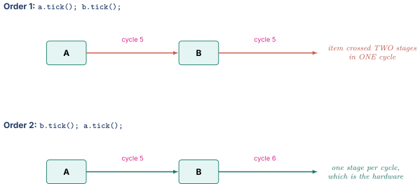
Order 1: a.tick(); b.tick(); A sees B is empty, hands the item over, sets B's valid_ to true. Then B's tick() runs, sees valid_ true (because A just set it this cycle) and sends the item downstream. The item traversed both stages in one cycle.
Order 2: b.tick(); a.tick(); B runs first, sees valid_ false, does nothing. Then A hands the item over. Next cycle B sends it. The item takes one cycle per stage.
Order 2 is what the hardware does. Order 1 is a combinational path straight through a register, which is not a thing that can exist in silicon.
Figure 3. The same two objects and the same state produce two different answers depending only on the order the model happened to call their tick methods, and only one of the two answers corresponds to hardware that could be built.
Now scale it. Three stages have six possible orders. Forty modules have 40!≈8×1047 orders, and the one you get is decided by insertion order into a std::vector, which is decided by the order somebody happened to write the constructor calls. The model is correct on the configuration you tested and becomes wrong the day a colleague adds a module in the middle. The symptom is a performance number that shifts by a few percent for no reason anyone can find, which is the worst possible symptom because it looks like noise.
That is the bug the two-phase discipline exists to prevent. Being able to tell that story concretely, in about ninety seconds, is a strong answer to a question that many candidates answer with "so that everything updates together," which is true and demonstrates nothing.
Split every module's per-cycle work into two methods with a strict contract.
C++
class Module{public:virtual ~Module()= default;// Phase 1. Read current state and neighbours' current outputs.// Compute what the next state should be and stash it privately.// WRITE NOTHING that another module can observe.virtual void evaluate()= 0;// Phase 2. Commit the stashed next state into current state.// READ NOTHING from any other module.virtual void update()= 0;virtual void reset(){}virtual void dumpStats(std::ostream&)const{}const std::string& name()const{return name_; }protected:std::string name_;};
The kernel becomes:
C++
void Model::advanceOneCycle(){
for(Module* m : modules_) m->evaluate(); // any order
for(Module* m : modules_) m->update(); // any order
++cycle_;
}
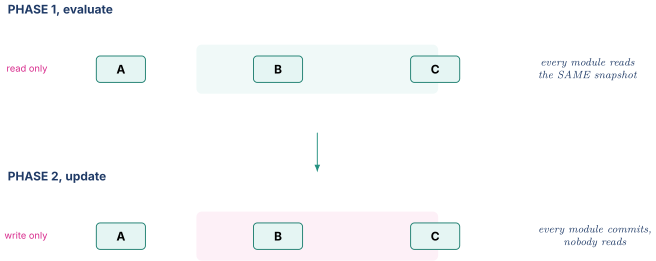
Why this fixes it. During evaluate, no observable state changes anywhere, so it does not matter who runs first. Every module sees the same snapshot, the state as of the start of the cycle. During update, nobody reads anything, so it does not matter who commits first. The result is provably independent of ordering within each phase, which means the 40! orderings collapse to one behaviour.
Figure 4. Splitting the cycle into a read-only phase and a write-only phase makes the order within each phase irrelevant, which is the same guarantee a non-blocking assignment gives in SystemVerilog and a delta cycle gives in SystemC.
This is the non-blocking assignment. In always_ff @(posedge clk) q <= d;, every right-hand side across the entire design is sampled from the pre-edge values, and every left-hand side is committed afterwards. SystemVerilog gives you that for free through the language's event region scheduling. C++ has no such construct, so a C++ hardware model has to implement it by hand, and that is what a hardware modelling framework fundamentally is. Saying that sentence in an interview is worth a great deal because it reframes the whole topic in terms the interviewer knows you know.
The implementation pattern is a two-valued register.
Read q() and d() as the flop's pins, which is not a coincidence.
The honest costs, because an interviewer will ask and "none" is not credible. This doubles the storage for every register, and it costs a copy per register per cycle even when nothing changed. For scalars that is nothing. For a 32 KB tag array it is emphatically not nothing, and you do not double it. Instead you keep the array single-valued and maintain a small journal of pending writes that update() applies, which costs one entry per actual write rather than one copy per entry per cycle. Knowing that the naive pattern does not scale to arrays, and knowing the journal fix, is exactly the kind of thing that separates having built one from having read the pattern.
The remaining hard case, which is worth raising unprompted. Some hardware signals genuinely are combinational across module boundaries within one cycle. A ready that propagates backward through three stages of a pipeline in the same cycle is the canonical one. Strict two-phase forbids that, because a ready computed in evaluate is not visible to anyone else until update. There are two clean resolutions. Iterate evaluate() to a fixed point, running it repeatedly until no output changes, which is precisely what SystemC's delta cycles do and what Part 6 describes. Or declare that module boundaries are register boundaries and forbid combinational crossing, handling backward-propagating ready signals with a credit or skid-buffer scheme instead, which is also, not coincidentally, what a well-partitioned RTL design does for timing-closure reasons, per Interconnect and AMBA. Most bespoke cycle models take the second option because it is simpler and because it forces the model's structure to match the RTL's, which makes correlation easier. Say which you chose and why. The choice is the answer, not the option.
A port is the same three-signal contract you already know from AXI-style channels in Interconnect and AMBA, expressed in C++ with the two-phase discipline built in.
Notice that the entire two-phase discipline is hidden inside the port. A module author writes if (out_.canSend()) out_.send(x); and cannot accidentally create the cycle-5 bug of 5.1, because there is no way to write a value that the consumer can observe this cycle. Encoding a discipline in a type so that violating it is not expressible is the single most valuable thing C++ gives you over C for this job, and it is a much better answer to "why C++" than "classes are nice."
For a single-clock model, the "clock" is a counter and 5.2's advanceOneCycle is the whole of it. The moment there is more than one clock, you need something better. A core at 3 GHz and a fabric at 1.5 GHz is the ordinary case.
The pragmatic answer is to keep a global tick counter in the finest unit you need, and have each module declare a period in those ticks.
That is simple, and it wastes work in exactly the way 2.1 describes when the ratio between the fastest and slowest clock is large. The scalable answer is to put the two-phase kernel inside an event-driven kernel. Each clock domain schedules one "advance domain" event per its own period, and that event runs the two phases for the modules in that domain. Now you have both properties (event-driven efficiency across domains, two-phase determinism within a domain), and that hybrid is, as far as I understand the public documentation, essentially the shape that both gem5 and SystemC arrive at, though the details differ and I would read the source before claiming any specific structural equivalence.
Two crossing-domain warnings that transfer directly from Clocking Reset and Domain Crossing. First, a model does not naturally reproduce metastability or synchroniser latency, so if the RTL has a two-flop synchroniser on a crossing and the model does not model those two cycles, you have built in a systematic two-cycle optimism on every crossing, which will show up in correlation as a constant offset. Model the synchroniser delay explicitly. Second, if the two domains are not integer-related, the model has to decide what happens at a non-aligned edge, and whatever it decides is a modelling assumption that needs writing down.
reset() exists so the model can be brought to a known state without reconstructing every object, which matters for warm-up (see Performance Modeling section 6.5) and for running many configurations in one process.
Statistics deserve more design attention than they usually get, because the statistics interface is the correlation interface. Part 8 consists almost entirely of diffing two sets of counters. Make them a registry with stable names.
C++
class Stats{public:uint64_t& counter(const std::string& name){return counters_[name]; }void dump(std::ostream& os)const{for(const auto&[name, value] : counters_) // std::map: sorted orderos << name << " = " << value << '\n';}private:std::map<std::string, uint64_t> counters_;};
std::map rather than std::unordered_map here is a deliberate and defensible choice, and it is worth being able to explain: the map is not in the hot path, it is dumped once at the end, and the ordered iteration means two dumps from two different runs are line-comparable with diff. Choosing the slower container because it makes the output diffable is a small decision that shows you were thinking about the workflow rather than the microbenchmark. Take the hot-path counter reference once at construction and hold it as a uint64_t& member so the per-cycle increment is a plain memory increment with no lookup at all.
Three conventions that will save you in Part 8. Name counters identically on both sides. If the RTL calls it l1d_primary_miss, the model calls it l1d_primary_miss, not primaryMisses. Define every counter in a comment at the point of declaration, stating exactly when it increments, because "when is a hit counted" is a real ambiguity that produces false discrepancies. And make the dump format one name = value per line, sorted, so the comparison tool is four lines of Python and not a parser.
SystemC is not a language. There is no SystemC compiler. It is a C++ class library plus a simulation kernel, distributed as source, that you #include and link against. Every SystemC program is a C++ program that a standard C++ compiler builds into an ordinary executable, and running the simulation means running that executable.
That is worth saying plainly because the name misleads people into expecting something like SystemVerilog. It is closer to what you would get if you took Part 5, wrote it very carefully, standardised it, and gave everyone the same one.
The standard is IEEE 1666. The long-standing revision was IEEE 1666-2011, which is the one most existing material references and which is also where TLM-2.0 was folded into the standard proper. The current revision is IEEE 1666-2023, with a Corrigendum 1 published in 2025. Accellera has made it available at no cost through the IEEE GET program. The 2023 revision moved the C++ baseline forward to a modern ISO C++ version and added capabilities aimed at co-simulation, including simulation-stage callbacks and a suspend mechanism. The reference implementation is Accellera's proof-of-concept library, distributed under Apache 2.0, and it is what almost everyone actually runs.
If you name a version in an interview, name 1666 and say "the 2023 revision is current, 2011 is the one most existing code targets," which is accurate and specific without over-claiming.
Six things, and it is worth knowing which of the six you actually care about.
A simulation kernel. The event queue of Part 2 and the two-phase discipline of Part 5, written, debugged, and standardised, with the ordering semantics specified in a document rather than in your head.
A time model.sc_time carries a value and a unit, so sc_time(10, SC_NS) is ten nanoseconds and not ten of something. There is a global time resolution, one picosecond by default. This eliminates a whole class of unit bugs that a raw uint64_t tick invites.
Structure.SC_MODULE, ports, exports, channels, and hierarchical instantiation, so a model has a described structure that tools can walk, rather than a graph of pointers only the author understands.
Hardware data types.sc_int<N> and sc_uint<N> for integers of any width up to 64 bits with the wraparound behaviour hardware has, sc_bigint/sc_biguint for widths past 64, sc_bv<N> for bit vectors, and sc_logic/sc_lv<N> for four-state values including X and Z. If you want a 37-bit counter that wraps like the RTL's, sc_uint<37> does it and uint64_t does not.
Concurrency. Processes that look like independent threads of control but are cooperatively scheduled by the kernel, so there is no preemption and no data races from the kernel's own scheduling.
TLM-2.0. A standard for transaction-level interoperability, which is 6.5 and is the reason large organisations use SystemC at all.
Here is the one-sentence case. SystemC buys you a standard answer to Part 5's questions instead of your own, and the value of that is almost entirely proportional to how much you need to plug into someone else's model. For a solo cache model, your own 400-line framework is arguably better because it is smaller and you understand every line. For an SoC virtual platform assembled from six teams' models plus two vendors' IP models, there is no serious alternative.
#include <systemc>using namespace sc_core;using namespace sc_dt;SC_MODULE(Counter){sc_in<bool> clk;sc_in<bool> rst_n;sc_out<sc_uint<8> > count;void step(); // the process bodySC_CTOR(Counter){SC_METHOD(step); // register step as a processsensitive << clk.pos(); // trigger on the rising edgedont_initialize(); // do not run once at time zero}private:sc_uint<8> count_ = 0;};void Counter::step(){if(!rst_n.read()) count_ = 0;else count_ = count_ + 1;count.write(count_);}
If you read that as always_ff @(posedge clk), you have read it correctly. The constructor's job is registration. It tells the kernel "call step whenever clk rises."
There are two process kinds and choosing between them is a real decision.
SC_METHOD runs to completion every time it is triggered. It cannot suspend, cannot call wait(), and has no stack of its own. It is cheap (a function call), which is why it is the right choice for anything triggered every cycle. Its analogue is an always block with a sensitivity list.
SC_THREAD has its own stack. It can call wait() in the middle of its body and resume from exactly that point when re-triggered, so you can write a bus protocol as straight-line sequential code: drive the address, wait() for the acknowledge, drive the data, wait(), done. Its analogue is a SystemVerilog task or an initial block with delays. Its cost is a coroutine context switch on every suspend and resume, which is far more than a function call, plus a stack per thread that has to be sized.
There is also SC_CTHREAD, a thread clocked on a single edge, which exists largely for the high-level-synthesis subset and which I would not reach for in a performance model.
The rule of thumb worth stating: SC_METHOD for anything in the per-cycle hot path. SC_THREAD when the logic is naturally a sequence and writing it as a state machine would obscure it. A model with a thousand SC_THREADs per cycle will be slow for a reason that has nothing to do with the modelling and everything to do with context switching, and that is a debugging story people tell.
sc_signal<T> is SystemC's implementation of exactly the two-valued register from 5.2. write() does not change what read() returns until the kernel says so. Here is the kernel loop that says so.
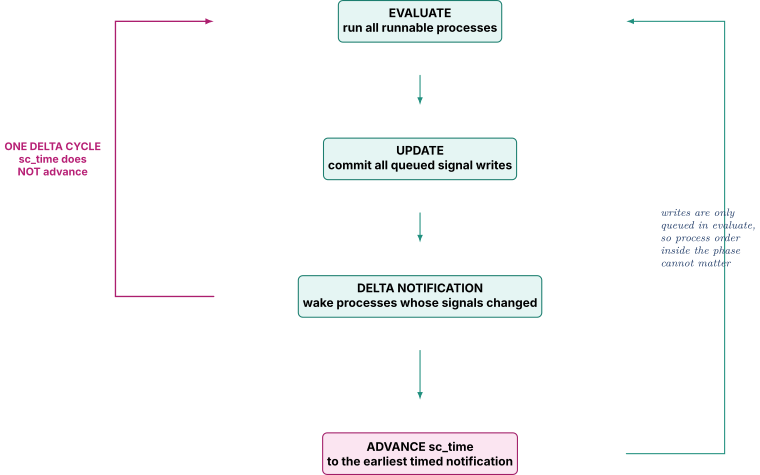
Figure 5. The SystemC kernel alternates an evaluate phase in which processes run and writes are only queued with an update phase in which those writes commit, and it repeats that pair without advancing time until nothing more changes, which is what a delta cycle is.
Walk it. In the evaluate phase the kernel runs every runnable process, in an order the standard deliberately leaves unspecified. Their write() calls do not take effect. They go onto an update list. In the update phase the kernel drains that list, committing every write. Signals whose value actually changed then notify their associated events. In delta notification, processes sensitive to those events become runnable. If any did, the kernel goes back to evaluate without advancing sc_time at all. That whole round trip is one delta cycle. Only when a full round produces no new runnable processes does the kernel advance sc_time to the next timed notification.
Two consequences you should be able to state.
A chain of combinational blocks settles over several delta cycles at the same simulated time. Three cascaded blocks take three deltas. That is the fixed-point iteration mentioned as option one in 5.2, done for you. It is also why sc_time_stamp() can return the same value many times in a row while things are visibly changing, which confuses everyone once.
The order of processes within the evaluate phase does not matter, by construction. The standard leaves it unspecified precisely because a correct SystemC model must not depend on it, and a model that does depend on it is broken in the 5.1 sense whether or not it currently produces right answers.
Here is the trap worth knowing, and it is the most common SystemC bug. sc_signal gives you the discipline, a plain C++ member variable shared between two processes does not. Mix them and you have silently reintroduced the order-dependence bug inside a framework that was supposed to prevent it, and the failure will be intermittent because it depends on the kernel's scheduling order. A related trap is sc_event::notify() with no argument, which is an immediate notification that makes processes runnable within the current evaluate phase rather than at the next delta. It is legal, it is occasionally necessary, and it destroys the order-independence guarantee, which is why the usual advice is to prefer notify(SC_ZERO_TIME), a delta notification, unless you have a specific reason. wait(SC_ZERO_TIME) is the corresponding idiom on the thread side, advancing one delta cycle without advancing time.
Two more constructs worth naming because they come up. sc_fifo<T> is a channel with blocking read() and write() and a bounded depth, which models a hardware FIFO with backpressure almost for free. sc_mutex and sc_semaphore exist for shared resources. And the top-level driver is sc_main, in which you instantiate the hierarchy, bind the ports, and call sc_start().
Moving a 64-byte burst across an AXI-style interface at RTL means dozens of signals changing over many cycles: address channel handshake, then eight or sixteen data beats each with its own valid and ready, then a response. An RTL simulator evaluates every one of those transitions, and every process sensitive to them. Call it a few thousand events for one cache line.
At transaction level, the same transfer is one function call: "write these 64 bytes to this address," carrying an annotation saying how long it should have taken. A few thousand events collapse to one call plus some arithmetic. That factor is why a virtual platform can boot an operating system in minutes while the RTL model of the same SoC would take weeks, which is the entire commercial reason SystemC exists at large companies.
The pieces.
Sockets.tlm_initiator_socket and tlm_target_socket. A socket bundles the forward interface (initiator to target) and the backward interface (target to initiator) so one bind() wires both directions. Sockets are what make two independently written models connectable.
The generic payload,tlm_generic_payload. One transaction object with a standard attribute set: a command (read, write, or ignore), an address, a data pointer, a data length, a byte-enable pointer and byte-enable length, a streaming width, a DMI-allowed hint, a response status, and an extension mechanism for protocol-specific fields the standard set does not cover. The whole point is interoperability. Two models from two organisations can exchange transactions because they agree on this object's shape, and protocol-specific needs go into extensions rather than into incompatible payload types.
The base protocol, which states which phase transitions are legal so that two models agree on the handshake as well as the data.
Two coding styles, and this is the part interviewers ask about.
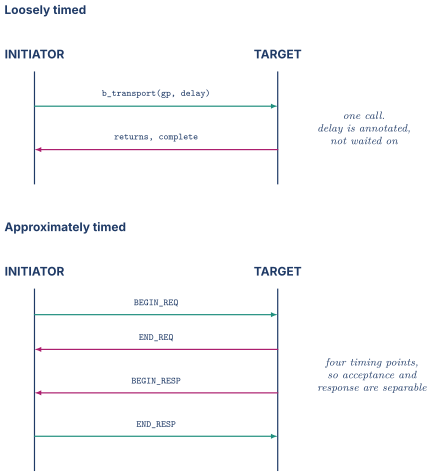
Loosely timed, LT. The initiator calls b_transport(payload, delay), a blocking call in which the entire transaction completes before the call returns. The delay argument is a timing annotation. The initiator accumulates it rather than actually suspending, which is the trick. Combined with temporal decoupling, where each initiator is allowed to run ahead of global simulated time by up to a global quantum managed by a tlm_quantumkeeper, and with DMI, the direct memory interface by which a target hands the initiator a raw pointer to a memory region so that subsequent accesses skip the transport call entirely, LT is fast enough to boot an OS. It is register-accurate and timing-suggestive.
Approximately timed, AT. The initiator calls nb_transport_fw and the target calls back on nb_transport_bw, breaking each transaction into phases. The base protocol defines four: BEGIN_REQ, END_REQ, BEGIN_RESP, END_RESP. Each transition is an explicit timing point, so request acceptance latency can be modelled separately from response latency, and multiple transactions can be in flight and pipelined against each other. The non-blocking calls return one of TLM_ACCEPTED, TLM_UPDATED, or TLM_COMPLETED to say how much of the phase transition the callee handled synchronously. AT is substantially slower than LT and still substantially faster than RTL.
Figure 6. Loosely timed collapses a whole transaction into a single blocking call with a delay annotation, while approximately timed exposes four phase transitions so that request acceptance and response can each carry their own timing.
The judgment sentence is what the question is really testing. Use LT when the consumer of the model is software, and AT when the consumer is an architect. A firmware team that needs to develop drivers against a model needs register accuracy and speed, so LT with DMI. An architect who needs to size a queue needs the model to say something honest about time, so AT.
And here is the caveat that shows you understand the limits, which is worth volunteering. LT numbers are not performance numbers. Temporal decoupling deliberately lets initiators run ahead of each other within the quantum, which means the interleaving of transactions from different initiators is not the interleaving the hardware would produce. If someone quotes you a bandwidth number from an LT model, the right response is to ask what the quantum was. Even AT is approximately timed by name. A genuinely cycle-accurate answer about one block usually means dropping below TLM to a signal-level or bespoke cycle model for that block while keeping TLM for everything around it, which is a normal and respectable architecture for a virtual platform.
Right. Virtual platforms that firmware develops against. SoC-level models assembled from many teams' pieces. Anywhere you must integrate a vendor's IP model, because vendors ship TLM-2.0. Anywhere the model has to outlive its author, because a standard structure is legible to the next person. And anywhere the group has already standardised on it. a fabric or last-level-cache modelling role naming SystemC explicitly is a strong signal that this is the case there.
Not right, or at least not obviously. A single-block cycle-accurate model where nothing external will ever connect to it. For the Part 7 cache, plain C++ with your own 400-line framework is smaller, faster, easier to correlate, and easier to explain, and the SystemC ceremony buys nothing because there is no second party to interoperate with. Being able to say "I'd use SystemC when interoperability or a virtual platform is the goal, and plain C++ when it's one block I need cycle parity on" demonstrates judgment rather than tool enthusiasm, and tool enthusiasm without judgment is a thing interviewers are specifically watching for.
There is one more honest note. SystemC's speed for a detailed, signal-level model is not obviously better than a well-written bespoke C++ model, because the kernel is doing general work that a bespoke model can specialise away. SystemC's speed advantage is overwhelmingly a TLM advantage. It comes from raising the abstraction level, not from the kernel being fast. Confusing those two is a common error and correcting it is a good thing to be able to do.
This ordering is not a stylistic preference. A cycle-accurate model is a claim about a specific design, so if the design is not written down, the model's claim is unfalsifiable and correlation is impossible. Write the spec, get it reviewed, then implement it twice, once in C++ and once in RTL, and the correlation study of Part 8 has something to be a study of.
Here is the specification. Every number is chosen so the arithmetic is clean, and nothing here is anyone's proprietary design. It is the ordinary textbook shape from Cache Organization and Prefetching.
Parameter
Value
Consequence
Capacity
32 KB
Line size
64 B
offset field is 6 bits
Associativity
8 ways
Sets
32768/64/8=64
index field is 6 bits
Write policy
write-back, write-allocate
dirty bit per line, writebacks on eviction
Hit latency
4 cycles, fully pipelined
one access accepted per cycle
MSHRs
8
at most 8 line fills outstanding
Targets per MSHR
4
at most 4 requests merged onto one fill
Fill latency
30 cycles, parameterised
from request issue to data return
Fill ports
1
a fill and a demand access conflict, and fill wins
Replacement
tree-PLRU, 7 bits per set
Writeback buffer
4 entries
a full buffer blocks the eviction
Address decomposition, worked on a real number. Take the physical address 0x0000_0000_1234_5678.
The low 6 bits are the byte offset within the line: 0x5678mod64. In binary the low twelve bits are 0110 0111 1000, so bits [5:0] are 111000, which is 56. The next 6 bits are the set index: bits [11:6] are 011001, which is 25. Everything above bit 11 is the tag: 0x12345.
\text{set} = (\text{addr} \gg 6) \;\&\; 63 = 25, \qquad
\text{tag} = \text{addr} \gg 12 = \texttt{0x12345}$$
Being able to do that decomposition on a whiteboard in under thirty seconds is table stakes for any cache question, per [Cache Organization and Prefetching](/learn/hardware-interview-prep/cache-organization-and-prefetching), and it is the first three lines of the model.
### 7.2 The state, and the single most consequential design choice in the file
```cpp
static constexpr uint32_t kLineBytes = 64;
static constexpr uint32_t kSets = 64;
static constexpr uint32_t kWays = 8;
static constexpr uint32_t kMshrs = 8;
static constexpr uint32_t kTargets = 4;
static constexpr uint32_t kWbEntries = 4;
static constexpr uint64_t kHitLat = 4;
static constexpr uint64_t kFillLat = 30;
struct Line {
uint64_t tag = 0;
bool valid = false;
bool dirty = false;
};
struct Target {
uint64_t seq = 0; // request sequence number, for the trace log
bool isWrite = false;
uint32_t offset = 0;
};
struct Mshr {
bool valid = false;
uint64_t lineAddr = 0;
uint64_t fillCycle = 0; // cycle the fill is expected
uint32_t numTargets = 0;
std::array<Target, kTargets> targets{};
};
class L1Cache : public Module {
public:
void evaluate() override;
void update() override;
void reset() override;
void dumpStats(std::ostream&) const override;
private:
std::vector<Line> lines_; // kSets * kWays, sized once
std::vector<uint8_t> plru_; // kSets entries, 7 bits used
std::array<Mshr, kMshrs> mshrs_{}; // FIXED SIZE. see below.
Fifo<uint64_t, kWbEntries> wb_; // writeback buffer
// ... ports, stats refs, cycle counter ...
};
```
Stop on `std::array<Mshr, kMshrs>`.
The hardware has eight MSHRs. Eight. It is a physical structure with eight sets of tag-comparison logic and eight state machines, and when all eight are busy the cache **stalls**. That stall is not an edge case. It is the mechanism that limits memory-level parallelism, and per [Cache Organization and Prefetching](/learn/hardware-interview-prep/cache-organization-and-prefetching) section 7.3 it is very often the actual limiter on memory-bound code, more often than DRAM bandwidth or latency.
If you write `std::vector<Mshr> mshrs_` and `push_back` on allocation, the model will never stall. It will silently model an infinite MSHR file. Every number it produces about memory-bound workloads will be optimistic, and it will be *most* optimistic exactly where the real machine hurts most. The model will look fine. It will pass every test you write. And it will be lying about the one thing you built it to measure.
**A fixed-size hardware structure must be modelled by a fixed-size container.** Not as a style preference, but as a correctness requirement, because the container's capacity *is* a modelling assumption. This generalises. A queue that can grow models a queue that never applies backpressure, and backpressure is where all the interesting behaviour is. If you take one implementation lesson from this note, take that one, and say it in interviews, because it is the kind of thing that only occurs to someone who has thought about what the model is *for*.
### 7.3 The tick, in evaluate-then-update form
The order of operations within `evaluate()` is itself a modelling decision and it must match the RTL. Write it down and comment it.
```cpp
void L1Cache::evaluate() {
// Order matters and mirrors the RTL's cycle:
// 1. Fills that land this cycle are processed first, because in the
// RTL the fill occupies the array port at the start of the cycle
// and frees its MSHR, which a demand access this cycle can then use.
// 2. Writeback buffer drain, which may free a writeback slot.
// 3. At most one new demand access is accepted, and only if the fill
// did not take the array port.
processFills();
drainWritebacks();
acceptDemand();
}
```
Every one of those three comments is a claim about the RTL that correlation will test. If the RTL actually frees the MSHR at the *end* of the cycle, then a demand access in the same cycle should *not* see it free, and the model is one cycle optimistic on every MSHR-full stall. That is a real, findable, one-cycle-per-event discrepancy, and it is exactly the kind of thing Part 8's first-divergence method catches.
`update()` then commits the ports and any journalled array writes, per 5.2.
<Figure src="/figures/hardware-interview-prep/iv-31-Cpp-and-Performance-Model-Construction-fig07.svg" alt="The cache model is one array of lines, one fixed-size MSHR file, one writeback buffer, and a set of counters, with the fill path and the demand path contending for a single array port each cycle." caption="The cache model is one array of lines, one fixed-size MSHR file, one writeback buffer, and a set of counters, with the fill path and the demand path contending for a single array port each cycle." id="fig:31-Cpp-and-Performance-Model-Construction-7" />
### 7.4 The hit path
```cpp
int L1Cache::findWay(uint32_t set, uint64_t tag) const {
const Line* s = &lines_[set * kWays];
for (uint32_t w = 0; w < kWays; ++w)
if (s[w].valid && s[w].tag == tag) return int(w);
return -1;
}
```
Two observations about that loop, and the second one is the interesting one.
First, it is $O(\text{ways})$, which for eight ways is eight comparisons and is cheap. Storing the tags contiguously per set (`set * kWays + w` rather than a vector of vectors) means all eight tags live in one or two cache lines of the *host* machine, so the loop is one host cache miss rather than eight. That is worth doing and costs nothing.
Second, and this is a good thing to volunteer in an interview. **The RTL does all eight comparisons in parallel in one gate delay. The model does them one after another.** That difference is invisible to the cycle count, which is the point of a cycle-accurate model. It gets the timing right without reproducing the mechanism. But it also means **the model is structurally blind to the cost of associativity**. Bumping the model from 8 ways to 16 ways costs eight more comparisons in a loop and changes the miss rate favourably, so the model will happily recommend 16 ways. Whether 16 ways of tag comparison and way-select muxing fits in the four-cycle hit latency at the target frequency is a question only [STA Synthesis and Physical Design](/learn/hardware-interview-prep/sta-synthesis-and-physical-design) and [SRAM Arrays and ECC](/learn/hardware-interview-prep/sram-arrays-and-ecc) can answer, and the model cannot even represent it. Naming that blind spot is the kind of thing your background lets you say and a pure-software modeller often cannot.
The hit itself:
```cpp
void L1Cache::onHit(uint32_t set, uint32_t way, const Request& r) {
Line& l = lines_[set * kWays + way];
if (r.isWrite) l.dirty = true;
plruTouch(set, way);
completeAt(r, cycle_ + kHitLat);
++stat_hits_;
if (r.isWrite) ++stat_writeHits_; else ++stat_readHits_;
}
```
### 7.5 The miss path and the MSHR file, which is where the model earns its keep
Four outcomes, in the order the logic must check them. The order is not arbitrary. It is the order the RTL checks them, and getting it wrong changes the counts.
```cpp
void L1Cache::onMiss(uint64_t lineAddr, const Request& r) {
// 1. SECONDARY MISS: an MSHR already covers this line.
if (Mshr* m = findMshr(lineAddr)) {
if (m->numTargets < kTargets) {
m->targets[m->numTargets++] = makeTarget(r);
++stat_secondaryMiss_;
return; // NO downstream request. This is the point.
}
++stat_targetFullStall_; // merged, but no room for another target
stall(r);
return;
}
// 2. PRIMARY MISS with a free MSHR.
if (int id = allocMshr(); id >= 0) {
Mshr& m = mshrs_[id];
m.valid = true;
m.lineAddr = lineAddr;
m.fillCycle = cycle_ + kFillLat;
m.numTargets = 1;
m.targets[0] = makeTarget(r);
issueDownstream(lineAddr, m.fillCycle);
++stat_primaryMiss_;
return;
}
// 3. PRIMARY MISS with no free MSHR: the cache blocks.
++stat_mshrFullStall_;
stall(r);
}
```
Three things to notice, each of which is a modelling decision with a correlation consequence.
**A secondary miss issues nothing downstream.** That is the whole reason MSHRs exist. Four accesses to four different words of the same 64-byte line cost one memory transaction, not four. If your merge condition is wrong (comparing full addresses instead of line addresses, say), the model issues four requests, quadruples downstream traffic, and reports a completely different `primaryMiss` count while the *sum* of primary and secondary stays the same. That specific signature is the worked example in Part 8, because it is one of the easiest bugs to make and one of the easiest to localise once you have both counters.
**`mshrFullStall` and `targetFullStall` are separate counters, deliberately.** They look similar and they lead to completely different RTL changes. `mshrFullStall` says "add MSHRs," which costs a wider CAM and more state machines. `targetFullStall` says "widen the target list," which costs a few more bits per MSHR and is far cheaper. Collapsing them into one "stall" counter throws away the information that decides which fix to fund. **Every counter should be defined so that its value points at a specific action**, and that is a principle worth stating generally.
**The stall path must be modelled, not skipped.** It is tempting to let a stalled request retry silently. In the RTL the request occupies the input port and back-pressures the load-store unit, per [Load Store and Memory Ordering](/learn/hardware-interview-prep/load-store-and-memory-ordering), and *that* is where the performance cost shows up. A model that lets stalled requests vanish is the growable-container mistake in a different costume.
The fill, when the scheduled cycle arrives:
```cpp
void L1Cache::processFills() {
for (uint32_t id = 0; id < kMshrs; ++id) {
Mshr& m = mshrs_[id];
if (!m.valid || m.fillCycle != cycle_) continue;
// ONE fill port, per the specification in 7.1. If a fill already took
// the array port this cycle, every other ready fill waits a cycle. Let
// this loop run unguarded and the model quietly grants itself as many
// fill ports as it has MSHRs, which is the first Category-1 divergence
// listed in 8.5 and is invisible until a burst of fills coincides.
if (arrayPortTaken_) {
m.fillCycle = cycle_ + 1;
++stat_arrayPortConflict_;
continue;
}
uint32_t set = setOf(m.lineAddr);
uint32_t way = plruVictim(set);
Line& v = lines_[set * kWays + way];
if (v.valid && v.dirty) {
if (wb_.full()) { ++stat_wbFullStall_; m.fillCycle = cycle_ + 1; continue; }
wb_.push(lineAddrOf(v.tag, set));
++stat_writebacks_;
}
v.valid = true;
v.dirty = false;
v.tag = tagOf(m.lineAddr);
plruTouch(set, way);
for (uint32_t t = 0; t < m.numTargets; ++t) {
if (m.targets[t].isWrite) v.dirty = true;
completeAt(m.targets[t], cycle_); // every target wakes at once
}
m.valid = false; // MSHR freed
arrayPortTaken_ = true;
}
}
```
There are two deferrals in that loop and both encode a physical limit. `arrayPortTaken_` is cleared in `update()` at the start of every cycle, so exactly one fill lands per cycle no matter how many MSHRs happen to come due together, which is what the specification's single fill port means. And note the second deferral, the one when the writeback buffer is full. The fill pushes itself one cycle later rather than dropping the writeback. That is what the hardware does and it is a real source of stall cycles under write-heavy workloads. A model that silently discards the writeback is optimistic in a way that will show up in correlation as a divergence that only appears on write-heavy traces, a diagnostic pattern worth recognising.
### 7.6 Tree-PLRU, small enough to hand-check
Eight ways. True LRU would need to record a full ordering of eight items, which is $\lceil \log_2 8! \rceil = \lceil \log_2 40320 \rceil = 16$ bits per set, and the update is a read-modify-write of all sixteen. Tree-PLRU approximates it with a binary tree of seven bits: one root, two at the next level, four at the next, with the eight ways as leaves.
Number the tree nodes so that node $i$ has children $2i+1$ and $2i+2$. Nodes 0 through 6 are the seven internal nodes and hold the seven bits. Nodes 7 through 14 are the leaves and correspond to ways 0 through 7. Convention: **bit 0 means the pseudo-LRU way is down the left child. Bit 1 means it is down the right child.**
```cpp
uint32_t L1Cache::plruVictim(uint32_t set) const {
uint8_t bits = plru_[set];
uint32_t node = 0;
for (int level = 0; level < 3; ++level)
node = 2 * node + 1 + ((bits >> node) & 1); // 0 -> left, 1 -> right
return node - 7; // leaves 7..14 -> ways 0..7
}
void L1Cache::plruTouch(uint32_t set, uint32_t way) {
uint8_t& bits = plru_[set];
uint32_t node = way + 7;
while (node != 0) {
uint32_t parent = (node - 1) / 2;
if (node == 2 * parent + 1) bits |= uint8_t(1u << parent); // came from
else bits &= uint8_t(~(1u << parent));// left/right
node = parent;
}
}
```
Hand-check it, because a policy bug is invisible in functional testing and shows up only as a miss-rate discrepancy.
Start with `bits = 0`. `plruVictim` walks $0 \to 1 \to 3 \to 7$, giving way 0. Now `plruTouch(set, 0)`. Node 7, parent 3, and $7 = 2\cdot3+1$ so we came from the left, set bit 3, giving `bits = 0b0001000`. Node 3, parent 1, came from left, set bit 1, giving `0b0001010`. Node 1, parent 0, came from left, set bit 0, giving `0b0001011`. Now `plruVictim` again. At node 0 the bit is 1, so go right to node 2. At node 2 the bit is 0, so go left to node 5. At node 5 the bit is 0, so go left to node 11, which is way 4.
Touching way 0 moved the victim pointer to way 4, the other half of the tree. That is the behaviour you want, and it took thirty seconds to verify. **Verify replacement policy by hand on a small case before you trust a miss rate**, because a subtly wrong PLRU produces plausible-looking miss rates that are simply wrong, and no functional test will flag it.
Seven bits versus sixteen, for a policy that is close to LRU in practice. That is the trade [Cache Organization and Prefetching](/learn/hardware-interview-prep/cache-organization-and-prefetching) describes, and being able to write both the victim and the touch function from memory is a reasonable interview ask.
### 7.7 The statistics, which are the reason the model exists
This is the section people skip and it is the section correlation runs on. Every counter below exists because some decision depends on it.
| Counter | Why it exists |
|---|---|
| `accesses`, `readAccesses`, `writeAccesses` | denominator for everything |
| `hits`, `misses`, split by read and write | the headline miss rate |
| `primaryMiss`, `secondaryMiss` | their ratio is your direct evidence of memory-level parallelism, and their sum must equal `misses` |
| `mshrFullStall` | says "add MSHRs" |
| `targetFullStall` | says "widen the target list", a much cheaper fix |
| `wbFullStall` | says "deepen the writeback buffer" |
| `arrayPortConflict` | contention for the single array port, both fill versus demand and fill versus fill, says "add a port", which is expensive, so you want to know it is real |
| `writebacks`, `dirtyEvictions` | downstream write traffic |
| `mshrOccupancyHistogram[0..8]` | **a histogram, not a mean.** A mean of 3.1 out of 8 tells you nothing about whether you spend 12 percent of cycles pinned at 8, which is the number that decides |
| `perSetAccesses[64]` | conflict hotspots, which is how you detect a pathological stride |
| `stallCyclesBySource` | the top-down accounting of [Performance Modeling](/learn/hardware-interview-prep/performance-modeling) Part 4, applied to one block |
Two rules about counters that are worth stating as rules.
**Every counter must have an RTL counterpart, or a plan for one.** A counter the RTL cannot produce is a counter you cannot correlate against, and by Murphy's law it will be the one you most want when a divergence appears. Design the counter set jointly across model and RTL, before either is written.
**Prefer histograms to means for occupancy.** A mean occupancy hides saturation, and saturation is the entire question you asked the model. This is the same argument as the difference between coverage and savings in [Power Fundamentals and Clock Gating](/learn/hardware-interview-prep/power-fundamentals-and-clock-gating) section 3.4. An aggregate that averages over the interesting regime tells you about the boring one.
### 7.8 What this model does not model, written down on purpose
A professional model ships with this list in its README. An amateur one does not have the list, which means the author has not thought about it, which means the numbers cannot be trusted at the edges.
**No wrong-path accesses.** Unless the model is driven by something that speculates, it sees only the correct path, and per [Performance Modeling](/learn/hardware-interview-prep/performance-modeling) section 2.4 that makes it optimistic about pollution and pessimistic about accidental prefetch, with no way to tell which dominates.
**No coherence and no snoops.** There is no external invalidation, no downgrade, no snoop occupying the tag port. Adding a second core would change everything, per [Cache Coherence Protocols](/learn/hardware-interview-prep/cache-coherence-protocols).
**No prefetcher.** So MSHR occupancy is demand-only, which understates pressure relative to a real machine, per [Cache Organization and Prefetching](/learn/hardware-interview-prep/cache-organization-and-prefetching) section 8.
**No physical timing, no area, no power.** 7.4's blind spot, and the reason the model cannot tell you whether the configuration it recommends is buildable.
**No banking.** The model has one array with one port. A real L1 is banked and the conflict pattern differs.
**No ECC and no error handling.** Which, given your doctoral work, is a place you could credibly extend it. Modelling the extra cycle an ECC correction costs on a read, and the read-modify-write on a partial write, is a small extension with a genuinely differentiated story behind it.
**Virtual versus physical indexing is assumed away.** The model takes physical addresses. A VIPT L1 has the aliasing constraints of [Virtual Memory and Memory Ordering](/learn/hardware-interview-prep/virtual-memory-and-memory-ordering) and the model does not represent them.
Writing that list is not an admission of weakness. It is the thing that makes the correlation number in Part 8 believable, for the reason 8.7 explains.
---
## Part 8, correlation, which is the deliverable that closes the gap
### 8.1 The claim you are trying to earn the right to make
[Performance Modeling](/learn/hardware-interview-prep/performance-modeling) Part 7 introduces correlation as the RTL engineer's half of performance work and gives the general method and the three discrepancy categories. This part specialises all of it to the case at hand (a model you wrote against RTL you wrote) and adds the part note 24 does not cover, which is how to write the study up so that it functions as a hiring artefact.
The target sentence, from 1.3:
> "I wrote a cycle-accurate C++ model of an 8-way non-blocking L1 with an 8-entry MSHR file, wrote the RTL for the same specification, ran both against the same traces through Verilator, and correlated them to within 1.4 percent on cycle count. The write-up has a divergence log with six entries. Two of them turned out to be bugs in my RTL, not in the model."
Every clause in that sentence is checkable, and an interviewer who wants to check it will ask about the divergence log. That is fine, because the divergence log is the good part.
### 8.2 What to correlate against, when you do not have an employer's RTL
Three options, in increasing order of value and effort.
**Against gem5's classic cache.** Easiest and weakest. gem5's cache is itself a cycle-approximate model, so agreeing with it proves you agree with another model, and disagreeing with it proves nothing about which is right. Useful as a sanity check, not as the deliverable.
**Against an open-source RTL core's cache.** More work, more credibility, and it chips at the RISC-V gap at the same time. The friction is that somebody else's cache has a specification you have to reverse-engineer from the RTL, which is exactly the anti-pattern [Verification Methodology](/learn/hardware-interview-prep/verification-methodology) section 2.4 warns about. If you write the model by reading the RTL, a shared misunderstanding produces the same wrong answer twice and the comparison passes with the bug invisible.
**Against RTL you wrote yourself, from the same written specification.** This is the recommendation, and for you specifically it is close to ideal.
Look at why it is the right choice rather than the lazy one. The independence problem is handled properly if you write the **specification** first, then the model, then the RTL, each from the spec. That is exactly the reference-model independence discipline of [Verification Methodology](/learn/hardware-interview-prep/verification-methodology) section 2.4, and you can say so in those words. The RTL half is your strongest skill, so half the project is on home ground and finishes fast. The whole thing is demonstrably yours, with no ambiguity about what you did. And it produces an artefact that **only** someone who can do both halves could produce, which is a much rarer profile than "can write C++" or "can write RTL" separately.
The practical shape: write the spec of 7.1, implement the C++ of Parts 5 and 7, implement the same thing in SystemVerilog, compile the RTL with **Verilator** into a C++ model per [Lab: The Open-Source HDL Workflow](/learn/computer-architecture/lab-hdl-workflow) and [Programming and Tooling](/learn/hardware-interview-prep/programming-and-tooling) section 3.1, drive both from the same trace file, and diff the outputs. Verilator is the right choice here for two reasons beyond speed: it produces a C++ class you drive from a C++ harness, so the two sides run in one process from one trace with no file-format skew, and writing that harness is itself real C++ in exactly the sense these roles mean.
### 8.3 The instrumentation, and the definitional traps that produce fake bugs
Both sides need identical counters with identical names and, far more importantly, **identical definitions**. Write the definitions down in the specification, because every one of the following ambiguities produces a Category-3 discrepancy ("both are right and the comparison is unfair"), and Category 3 is the most common and most embarrassing outcome of a first correlation run.
**When is a hit counted?** At the cycle the access is accepted, or at the cycle the data is returned four cycles later? Those differ by four cycles times the hit count, which on a 100,000-access trace is 400,000 cycles of pure definitional gap.
**Does `accesses` include stalled retries?** If a request stalls on MSHR-full and retries next cycle, is that one access or two? The model and the RTL will make opposite choices if nobody decides.
**Are line-crossing accesses one or two?** An 8-byte load at offset 60 touches two lines. One access or two? Both answers are defensible. Only one can be in force.
**Where does the cycle counter start?** At reset release, at the first request, or at the first request after a warm-up phase? Note 24 section 7.3 lists this as the classic constant-offset signature.
**Does a writeback count as an access?** It uses the array port, so from a contention standpoint it behaves like one.
The other half of instrumentation is a **per-access trace record**, emitted by both sides in the same format, because aggregate counters localise a divergence to a structure and the per-access log localises it to an instant.
```text
seq cycle_accepted cycle_completed op addr result way mshr stall
0 12 16 R 0x1234_5678 HIT 3 - -
1 13 47 R 0x1234_5700 MISS_P 5 0 -
2 14 47 R 0x1234_5708 MISS_S - 0 -
3 15 15 W 0x1234_5710 STALL - - MSHR_FULL
```
Emitting that from the model is trivial. Emitting it from RTL means a few extra signals brought out to the Verilator harness, which is ordinary DFT-style observability work of the kind [DFT and Silicon Debug](/learn/hardware-interview-prep/dft-and-silicon-debug) describes, and which you have done.
### 8.4 The method, in four steps that must happen in order
**Step 1, prove comparability before proving anything else.** Run a ten-access hand-written trace through both sides and demand an **exact** match, cycle for cycle, on every line of the per-access log. Not "close." Exact. If a ten-access trace does not match exactly, no longer trace will teach you anything, because you will be unable to distinguish real divergences from definitional skew. This step feels like a waste of an afternoon and it is the single highest-return afternoon in the project.
**Step 2, aggregate cycle count, with the tolerance stated in advance.** Decide before you look at the number what counts as correlated. Three percent mean absolute percentage error across the suite is a defensible target for a first model of a single block. Deciding afterward is how people talk themselves into a number.
**Step 3, event counts side by side.** One table, every counter, both sides, absolute delta and percentage delta. This localises a discrepancy to a *structure* without a single waveform, and it is astonishingly effective. Note 24's section 7.2 makes the general case. Here is the specialised version and a worked example.
Suppose total cycles differ by 6.3 percent. You look at the counter table:
| Counter | Model | RTL | Delta |
|---|---|---|---|
| `accesses` | 100,000 | 100,000 | 0 |
| `hits` | 91,240 | 91,240 | 0 |
| `misses` | 8,760 | 8,760 | 0 |
| `primaryMiss` | 3,102 | 5,251 | **+69%** |
| `secondaryMiss` | 5,658 | 3,509 | **-38%** |
| `mshrFullStall` | 1,204 | 4,880 | **+305%** |
| `writebacks` | 2,890 | 2,890 | 0 |
Read it. Total accesses, hits, and misses match exactly, so the two caches agree completely about *what* is in the cache. The tag logic and the replacement policy are identical. But the split of misses into primary and secondary differs sharply while the **sum is identical**, $3102 + 5658 = 5251 + 3509 = 8760$. Requests that the model merged onto an existing MSHR, the RTL treated as new primary misses. More primary misses means more MSHRs allocated, which means the file saturates more often, which is exactly the `mshrFullStall` explosion, which is exactly the cycle gap.
**In one table, with no waveforms, you have localised the bug to the secondary-miss merge condition.** The most likely cause is an address comparison at the wrong granularity, comparing full addresses rather than line addresses, so two accesses to different words of the same line fail to merge. That is a bug in whichever side is wrong, and now you know exactly which twenty lines to look at on both sides.
That worked example is worth memorising as a *pattern*. **When two counters move in opposite directions and their sum is invariant, the bug is in the logic that classifies between them.** It generalises far beyond caches.
**Step 4, first divergence in the per-access log.** When counters do not localise it, diff the two per-access logs and find the **first** row where they differ. Everything after it inherits the offset and is not independent evidence. Look at that one access, look at what the RTL waveform shows it waiting for, and explain that single instant.
Here is the discipline point, and it is the one people violate. **Fix one divergence at a time and rerun the whole suite.** Fixing three things at once and getting a match tells you nothing about which fix was correct, and it is entirely possible that two of your three "fixes" were compensating errors that will diverge again the moment the workload changes.
### 8.5 The discrepancy categories, specialised to this model
Note 24 section 7.3 gives the three categories. Here is what each looks like for the Part 7 cache, which is the level of concreteness an interviewer is fishing for.
**Category one, the model is wrong.** The most common outcome, and not a failure, because a model that captured everything would be the RTL. Realistic instances are easy to name. The model let two fills land in the same cycle when the RTL has one fill port. The model updates PLRU at access time while the RTL updates it at fill time, so the victim sequence diverges after the first miss. The model treats a write hit to a clean line as one cycle while the RTL takes two, because setting the dirty bit is a read-modify-write of the state array. The model frees an MSHR at the start of the fill cycle while the RTL frees it at the end. Every one of those is a one-line fix and a real cycle-count difference. The consequence to state is that **every projection made with the old model is now suspect**, which is why finding a model error late in a project is genuinely expensive.
**Category two, the RTL is wrong, and it is usually a performance bug, not a functional one.** This is the class [Performance Modeling](/learn/hardware-interview-prep/performance-modeling) section 7.4 defines: correct results, delivered slowly, invisible to every scoreboard and assertion in [Verification Methodology](/learn/hardware-interview-prep/verification-methodology). The cache-specific instances are just as concrete. MSHR-full asserts at seven of eight because of an off-by-one in the comparison, so you built eight and deployed seven. The secondary-miss merge compares the wrong address bits, so every secondary miss issues a redundant downstream request and downstream traffic doubles while results stay perfect. The PLRU update is dropped on the fill path, so the tree degrades toward round-robin and the miss rate rises by a percent nobody can explain. The writeback buffer's full signal is registered, so it asserts a cycle late and the fill path stalls unnecessarily.
Notice that **two of those are exactly the bug in the 8.4 worked example, from the two possible sides.** Which side is wrong is decided by reading the specification, not by assuming the RTL is right or that the model is.
**Category three, the comparison is unfair.** The definitional list in 8.3, plus warm-up state and counter start conditions. Step 1 exists to eliminate this category before it wastes a week.
### 8.6 How to write the study up
A correlation study is a document with a fixed shape, and following the shape is most of what makes it read as professional. Ten sections.
**1, Scope.** What was modelled, at what abstraction, against what reference, and what question the model exists to answer. Two paragraphs.
**2, Configuration.** Every parameter of both sides in one table, so the result is reproducible. The table in 7.1 is this section.
**3, Stimulus.** The traces: where they came from, how long, what access patterns they contain, and why those and not others. If they are synthetic, say so and say what each was designed to stress. Take a stride trace, a pointer-chase trace, a write-heavy trace, and a trace with a working set that just fits and one that just does not. That set of four exercises most of the interesting behaviour and takes an afternoon to generate.
**4, Comparability proof.** The ten-access exact match from step 1, plus the counting-convention table. This section is short and it is the one that makes a skeptical reader relax.
**5, Aggregate result.** Per-trace cycle counts, model, RTL, delta, percentage. Then the summary statistic, **explicitly named**: mean absolute percentage error, and separately the worst case. Quoting one without the other is the thing that gets caught.
**6, Event-count table.** Every counter, both sides, all traces. Long and boring and the reason section 7 is credible.
**7, Divergence log.** One entry per divergence found, each with: the symptom, the evidence that localised it, the root cause, the category, the resolution, and the before-and-after numbers. **This is the section a reviewer actually reads and it is the section that proves you did the work.** Anyone can write a model. Only someone who drove a model to agreement with an implementation has a divergence log.
**8, Remaining known divergences.** With magnitudes, and why each was accepted rather than fixed. "Trace 7 remains 3.1 percent off because the model does not represent the writeback buffer's arbitration against fills, and fixing it was judged not worth the complexity for the questions this model answers" is a *good* sentence.
**9, Limitations.** Section 7.8's list.
**10, Reproduction.** How to build both sides and rerun everything, in enough detail that someone else could.
Length: eight to fifteen pages including tables. Publish it somewhere linkable (a repository README, a page on your own site), because a link in a resume that resolves to a document with a divergence log in it does more work than any bullet point could.
### 8.7 Why the limitations section makes the number more believable, not less
There is a counterintuitive dynamic here worth understanding, because it changes how you present the whole thing.
A correlation study reporting 0.4 percent error with no limitations section reads as either naive or dishonest, and an experienced reader's first instinct is to look for what was swept under the rug. A study reporting 1.4 percent mean, 3.1 percent worst case, with six divergences documented and three known limitations remaining, reads as **true**, and true is what you are selling.
The same asymmetry holds in the room. Compare two answers to "how accurate was your model?"
*"It correlated within half a percent."* The follow-up is "against what, on what stimulus, and how did you define the error," and if any of those answers is thin, the whole claim collapses and takes your credibility with it.
*"Mean absolute error of 1.4 percent across four traces, worst case 3.1 percent on the write-heavy one. I know exactly why that one is worst. I don't model the writeback buffer's contention with the fill path, so a burst of dirty evictions looks free in the model. I could have fixed it in about a day but it doesn't affect the question I built the model to answer."*
The second answer is worth several times the first, and it is worth it precisely **because** it names a weakness. It demonstrates that you measured, that you understood the residual, that you made a scoping decision deliberately, and that you can hold a number and its caveats in the same sentence. That is the behaviour of someone who has shipped a model, and it is not fakeable by someone who has not.
---
## Part 9, gem5 in context, and where a bespoke model wins
### 9.1 gem5's kernel is Part 2, which is the whole trick to talking about it
[Performance Modeling](/learn/hardware-interview-prep/performance-modeling) section 2.5 introduces gem5 as the standard open-source execution-driven simulator and [Lab: gem5 Out-of-Order Modeling](/learn/computer-architecture/lab-gem5-ooo) is the hands-on lab. What that material does not do is connect gem5's internals to the event-queue material, and that connection is what makes "have you used gem5" answerable with substance.
gem5 is an event-driven simulator built on exactly the structure of Part 2. Time is measured in **Ticks**. Events live in an **EventQueue**, and the top-level `simulate()` function runs a loop (`doSimLoop`) that repeatedly takes the earliest event off the queue and executes it. Hardware components are **SimObjects**, configured in Python and implemented in C++, and they communicate through **Ports**. A SimObject that wants to do something later calls `schedule()` with a target Tick. Events carry a **priority** field so that same-tick ordering is specified rather than accidental, which is 2.4's problem solved the same way.
If you can say that paragraph, you have said the useful part of "I understand gem5's architecture," and it is verifiable from the public documentation and source, which means you can say it honestly after an afternoon of reading rather than a year of use.
### 9.2 What gem5 gives you that you would otherwise build
**Real execution, therefore real behaviour.** Syscall-emulation or full-system mode means the model runs actual programs, which means it speculates, goes down wrong paths, and squashes, recovering everything a trace-driven model structurally cannot represent, per [Performance Modeling](/learn/hardware-interview-prep/performance-modeling) section 2.4.
**ISA models.** Several, so you are not writing a decoder.
**Two memory systems.** The "classic" memory system for speed and simplicity, and Ruby for detailed coherence protocol modelling, which matters for anything in [Cache Coherence Protocols](/learn/hardware-interview-prep/cache-coherence-protocols) territory.
**A statistics framework, checkpointing, and a configuration language**, all of which you would otherwise build badly.
**Community and prior art.** Someone has already made and fixed the mistakes you are about to make.
### 9.3 The three reasons teams still write bespoke models
This is the judgment question, and "just use gem5" is the wrong answer as reliably as "never use gem5" is.
**Fidelity for one specific block.** gem5's classic cache is cycle-approximate by design. If you need cycle parity with a *particular* cache that has a *particular* pipeline, a *particular* fill-port arbitration, and a *particular* MSHR allocation policy, you need a model shaped like that cache. Bending a general framework into that shape is frequently more work (and much harder to reason about) than 1,500 lines of your own code that does exactly one thing. This is the reason the Part 7 model exists as a standalone artefact rather than a gem5 patch.
**Speed for one specific question.** A sweep of forty MSHR configurations against a fixed address trace does not need an ISA model, a syscall layer, or a memory image. A bespoke trace-driven model runs orders of magnitude faster and answers the question the same afternoon rather than the same fortnight. The general-purpose simulator's generality is a cost you pay on every run.
**Instrumentation symmetry for correlation.** Part 8 lives on having counters on both sides with matched definitions. Adding a counter to your own 1,500 lines takes two minutes. Plumbing a new statistic through a large framework's stats infrastructure, in a form that matches what the RTL emits, takes considerably longer and is a place where subtle definitional mismatches creep in.
A fourth, which applies in industry and which you should phrase carefully: a model of a design that a general simulator has no shape for. Stated generically and without reference to any employer's internals, when the design departs structurally from what the framework assumes, the framework stops being a head start.
**The one-sentence rule: gem5 for questions about the machine, bespoke for questions about a block.** ROB sizing, branch predictor comparisons, workload characterisation, and anything that needs real programs all go to gem5. Cycle parity with one RTL block, a fast parameter sweep, and anything that will be correlated all go to bespoke.
### 9.4 Verilator, the third option people forget
Verilator compiles synthesizable SystemVerilog into a C++ class. That class **is** a cycle-accurate model. It just happens to have been generated from RTL rather than written by hand, and it is the fastest open-source route to running RTL at speed. Be precise about the sense in which it is cycle-accurate, because the qualifier matters and volunteering it is free. Verilator is two-state and settles the design once per evaluation rather than modelling intra-cycle time, so it reproduces the RTL's cycle-by-cycle behaviour for synchronous logic and reproduces nothing at all about X propagation, glitches, or delay-annotated timing. For the correlation of Part 8, where the question is only ever "how many cycles," that is exactly the right trade. For the X-propagation questions of [Verification Methodology](/learn/hardware-interview-prep/verification-methodology) it is the wrong tool and an event-driven four-state simulator is the right one.
Three consequences worth knowing. It is how you get the RTL half of Part 8 running fast enough to be useful. Writing the harness that instantiates the generated class, toggles the clock, drives stimulus from a trace, and reads back counters is genuine C++ in exactly the context these roles mean, which is the point [Programming and Tooling](/learn/hardware-interview-prep/programming-and-tooling) section 3.3 already makes. And it reframes the whole "C++ versus RTL" framing. For a design that exists, the fastest C++ model available is often the one the RTL compiler generated, and the hand-written model earns its keep by being faster still, by existing *before* the RTL, and by being cheap to change.
---
## Part 10, the data structures and algorithms that live inside these loops
### 10.1 Why these roles screen on this at all
Several of the eight role descriptions put a software-style coding screen in front of the architecture interview, and candidates from a hardware background often treat it as an unrelated hoop. It is not unrelated. Look at what the model in Parts 2 through 7 is actually made of.
| Structure in the model | The interview canon it is |
|---|---|
| the event queue | a binary heap / priority queue |
| MSHR lookup by line address | an associative lookup, hash map or small CAM scan |
| LRU ordering | hash map plus doubly-linked list |
| every hardware queue and FIFO | a ring buffer |
| address decomposition, free-entry search | bit manipulation |
| sizing sweeps | binary search on a monotone predicate |
The screen is a proxy for whether you can build the thing. Framed that way it stops being a hoop and becomes the same subject.
There is also a presentation advantage available to you that most candidates do not have. When you solve one of these, **name the hardware structure it is**. "This is a min-heap, and it is the same thing as the event queue in a discrete-event simulator." "This is a ring buffer with a power-of-two capacity, which is why I can mask instead of taking a modulo, and it is exactly a hardware FIFO with the extra-bit full/empty trick." That habit takes two seconds, costs nothing, and marks you as someone with a distinctive angle rather than a slower version of a software candidate.
### 10.2 The binary heap, built by hand
A **min-heap** is an array with one property. For every element, the element is $\leq$ both of its children. It is drawn as a tree but stored as a flat array, and the tree structure is arithmetic rather than pointers. Element $i$ has children at $2i+1$ and $2i+2$ and parent at $\lfloor (i-1)/2 \rfloor$.
Work it by hand. Insert 5, 3, 8, 1 into an empty min-heap.
| Operation | Array after | Reasoning |
|---|---|---|
| insert 5 | `[5]` | first element, nothing to compare |
| insert 3 | `[3, 5]` | 3 goes to index 1, parent is index 0 holding 5, and $5 > 3$ so swap |
| insert 8 | `[3, 5, 8]` | 8 goes to index 2, parent is index 0 holding 3, and $3 < 8$ so stop |
| insert 1 | `[1, 3, 8, 5]` | 1 at index 3, parent index 1 holds 5, swap to give `[3,1,8,5]`, then at index 1, parent index 0 holds 3, swap to give `[1,3,8,5]` |
Now pop the minimum. Take the root, 1. Move the last element, 5, to the root, giving `[5, 3, 8]`. Sift it down. The children of index 0 are index 1 holding 3 and index 2 holding 8. The smaller is 3, and $5 > 3$, so swap, giving `[3, 5, 8]`. Index 1 has no children, so stop. Result: returned 1, heap is `[3, 5, 8]`.
Both operations touch one root-to-leaf path, which is $\lfloor \log_2 n \rfloor$ levels, so both are $O(\log n)$.
<Figure src="/figures/hardware-interview-prep/iv-31-Cpp-and-Performance-Model-Construction-fig08.svg" alt="A binary heap is stored as a flat array and the tree is pure arithmetic, so element i has children at 2i+1 and 2i+2 and there are no pointers, no allocation, and perfect locality." caption="A binary heap is stored as a flat array and the tree is pure arithmetic, so element i has children at 2i+1 and 2i+2 and there are no pointers, no allocation, and perfect locality." id="fig:31-Cpp-and-Performance-Model-Construction-8" />
The array representation is not an optimisation detail, it is most of the point: no allocation per node, no pointer chasing, and a root-to-leaf walk touches $\log n$ elements that are increasingly far apart but all inside one contiguous block. That is why a heap beats a balanced tree in practice for this job even though both are $O(\log n)$.
In C++ this is `std::priority_queue`, which is a heap over a `std::vector`. Two facts get asked. It is a **max**-heap by default, so a min-heap of events needs a comparator that reverses the sense, which is exactly what `LaterFirst` in 2.3 does, and the reason it reads backwards on first sight. And it does not let you modify or remove an arbitrary element, which matters because a hardware model sometimes needs to cancel a scheduled event. The standard workaround is **lazy deletion**, where you mark the event dead and skip it when it pops, and that is what you should say if asked.
### 10.3 Hash maps, and the observation that a cache is one
Do it on numbers first. Take four buckets, numbered 0 to 3, and the trivial hash `key % 4`. Store key 17: $17 \bmod 4 = 1$, so it goes in bucket 1. Store key 6: $6 \bmod 4 = 2$, bucket 2. Store key 9: $9 \bmod 4 = 1$, which is bucket 1 again, where 17 already sits. That is a **collision**, and everything interesting about hash maps is what you do about it. Store key 13: $13 \bmod 4 = 1$ as well, so bucket 1 now wants to hold three keys in a structure that was drawn with one slot per bucket. Looking up 9 means going to bucket 1 and then searching within it, so the cost of a lookup is one arithmetic operation plus however deep that bucket got.
Generalise from exactly that. A hash map is an array of buckets. To store a key you compute `hash(key) % numBuckets` and put it in that bucket. Collisions, two keys landing in the same bucket as 17 and 9 did, are resolved either by **chaining**, keeping a list per bucket, or by **open addressing**, probing subsequent slots until an empty one is found. Lookup is $O(1)$ on average and $O(n)$ in the worst case where everything collides into one bucket, which is the four-keys-in-bucket-1 case taken to its limit.
Now the observation worth carrying into an interview. **A set-associative cache is a hash table.** The set index is the hash function, specifically the *line* address modulo the number of sets, `(addr >> 6) & 63` for the 64-set cache of 7.1, which is a modulo by a power of two and so the cheapest possible hash. Note that it is the line address and not the raw byte address, because the six offset bits have to come off first or every byte of a line would hash to a different set. The ways of a set are the bucket. The associativity is the bucket depth. And a **conflict miss** is what happens when a fixed-depth bucket overflows and something has to be thrown away (bucket 1 above holding only two of its four keys), which is the one thing a software hash table never does and a hardware one always does.
That reframing costs one sentence and reframes an entire topic, and it also answers a question that gets asked in both directions. The question "why is a cache set-associative rather than fully associative" is the same question as "why does a hash table have buckets rather than one big linear scan."
The C++ judgment question, "when would you *not* use a hash map in a model," has a crisp answer from 4.8. When the key is a small dense integer, use an array and index it. A tag array indexed by set number wants `lines_[set * kWays + way]`, which is a multiply and an add, against a hash, a modulo, a bucket dereference, and a chain walk. Reach for `std::unordered_map` only when the key space is genuinely sparse. A simulated memory image keyed by address is the canonical and nearly the only case in a hardware model.
### 10.4 LRU in software versus LRU in hardware, which differ and should
The classic problem is to implement a cache with $O(1)$ `get` and `put` and LRU eviction. The standard answer is a hash map from key to a node, plus a **doubly-linked list** ordering nodes by recency. `get` finds the node through the map and splices it to the front of the list. `put` inserts at the front and, when over capacity, drops the tail. Both are $O(1)$ because the map gives direct access to the node and a doubly-linked list can unlink a known node in constant time without traversal.
The performance-conscious version makes the list **intrusive**, meaning the previous and next pointers live inside the value object rather than in a separate list node. That removes one allocation per element and one pointer chase per traversal step.
Now the part that is yours to say. **Real caches do not implement true LRU**, for the reason 7.6 gives. Eight ways of true LRU means recording a full permutation of eight items, $\lceil \log_2 8! \rceil = 16$ bits per set, updated as a read-modify-write on **every access including hits**, which is a write to the state array on the critical path of the most common operation in the machine. Tree-PLRU does it in seven bits with a much cheaper update and gets most of the benefit.
So the software answer and the hardware answer to "implement LRU" are different, and they are different for a reason you can articulate. In software the constraint is asymptotic complexity and allocation, and in hardware the constraint is bits of state and the write port on the critical path. Being able to give both answers and explain why they diverge is a genuinely strong two minutes.
### 10.5 The ring buffer, which is every hardware queue
Fixed-capacity array, a head index, a tail index, and either a count or the extra-bit trick from [Arbiters FIFOs and CAMs](/learn/hardware-interview-prep/arbiters-fifos-and-cams) to distinguish full from empty when head equals tail. The `Fifo` template in 4.6 is exactly this.
Two details that come up. **Power-of-two capacity lets you mask instead of taking a modulo**, `(i + 1) & (Depth - 1)` rather than `(i + 1) % Depth`, which matters both because division is slow on a host CPU and because it is the same reason hardware queue depths are powers of two. And **the full-versus-empty ambiguity** is a real problem with a real hardware solution. With $N$ entries and $\log_2 N$-bit pointers, head equals tail in both the full and empty states, so you either keep a separate count, or waste one entry, or make the pointers one bit wider and compare the extra bit. That last one is the trick the asynchronous FIFO in [Whiteboard and Coding Playbook](/learn/hardware-interview-prep/whiteboard-and-coding-playbook) section 3.4 uses, and mentioning it in a software interview is a small, memorable flourish.
### 10.6 The bit manipulation you will actually use
Address decomposition is `addr >> 6` and `addr & 63`, and those two are in the first three lines of any cache model.
Finding the first free MSHR from a valid bitmask is `__builtin_ctz(~valid_mask)`, count trailing zeros. Be precise about what that costs, because it is the kind of detail an Apple interviewer is entitled to poke at. On x86-64 it is one instruction, `TZCNT` where BMI1 is available and `BSF` otherwise. On AArch64 there is no baseline trailing-zero instruction at all. The compiler emits `RBIT` to reverse the bits and then `CLZ` to count leading zeros, so it is two. A scalar `CTZ` instruction does exist, but only on cores implementing FEAT_CSSC, which arrived with Armv8.9 and Armv9.4, and the architecture reference defines it as leading-zero-count of the bit-reversed operand anyway. Either way it is a couple of cycles rather than a loop, and it is worth saying out loud that **this is a priority encoder**, the exact structure of [Arbiters FIFOs and CAMs](/learn/hardware-interview-prep/arbiters-fifos-and-cams), and that the reason the CPU has an instruction for it is the same reason the cache has the circuit for it.
`popcount(x)` counts set bits and gives you occupancy from a bitmask directly, one `POPCNT` instruction on x86-64 and, on baseline AArch64, a short SIMD sequence rather than a scalar instruction. `x & (x - 1)` clears the lowest set bit, so for a non-zero `x` the test `(x & (x - 1)) == 0` is a power-of-two test, which is the `static_assert` in 4.6. And the reason that assert also has to check `Depth != 0` is that zero passes the mask test and is not a power of two. `x & -x` isolates the lowest set bit.
The general point is that representing an 8-entry MSHR file's valid bits as a `uint8_t` bitmask rather than eight `bool`s makes allocation, occupancy, and full-detection each a single instruction, and it is also closer to what the hardware does. That alignment between "faster in the model" and "more like the RTL" happens often enough to be a heuristic.
### 10.7 The five to be able to write cold, and how to present them
**A binary heap** with push and pop. It is the event queue and you should be able to write both sift operations without hesitating.
**An LRU cache** with $O(1)$ get and put. Hash map plus doubly-linked list, and then the hardware footnote from 10.4.
**A ring buffer** with correct full and empty detection. Then the extra-bit variant.
**Binary search on a monotone predicate**, not on a sorted array. The model-shaped version of this is "find the smallest MSHR count that reaches 90 percent of peak throughput," where you have a function from configuration to result and you are searching for a threshold. It is the same algorithm and it looks nothing like the textbook framing, which is why it is worth having recognised in advance.
**A sliding window or two-pointer scan over a trace**, which is what every "compute the reuse distance" or "find the largest window with at most $k$ distinct lines" question actually is, and which is a real analysis you would run on a real address trace.
Two presentation habits that are worth more than a sixth algorithm. **State the complexity before you write the code**, in one sentence ("this is $O(n \log n)$ time and $O(n)$ space, dominated by the sort"), because it tells the interviewer you decided rather than stumbled. And **name the hardware analogue after you finish**, per 10.1. Neither takes ten seconds and both differentiate you from every other candidate in the queue.
---
## Part 11, interview questions with model answers
Sixteen questions, each with an answer written the way a strong candidate would actually speak it rather than the way a textbook would state it, the follow-up the interviewer will ask next, and, where the question is a trap, what the trap is.
Read the model answers out loud. They are written to be spoken, which means they are shorter and more concrete than written prose would be, and they lead with the thing the interviewer wants rather than building up to it.
### 11.1 "Explain how a discrete-event simulator works."
**Model answer.** "You keep a queue of things that are going to happen, each stamped with the simulated time it happens at, sorted earliest first. The main loop pops the earliest one, sets the current time to that event's timestamp, and runs it. Running it typically schedules more events, always at a time greater than or equal to now.
The key property is that time is data, not a loop counter. It jumps from one event to the next and skips everything in between, so the cost of the simulation is proportional to the number of events, not to the length of simulated time. That's why it beats a time-stepped loop for anything that's mostly idle. A DRAM bank that does something once every forty cycles costs you one event instead of forty function calls.
Implementation is a binary heap, so push and pop are logarithmic in the number of resident events, and in practice the queue is small so the heap isn't the bottleneck. The two things you have to get right beyond that are to assert that nothing ever schedules into the past, because that's a causality violation with no sensible recovery, and to make same-timestamp ordering a total order with an explicit rule."
**The follow-up: "Why does same-timestamp ordering matter?"** Answer it with the credit example from 2.4. Two events at tick 100, one returns a credit and one consumes it, counter is at zero. Consume-first underflows. Return-first is fine. With a timestamp-only comparator, which one you get depends on the heap's internal layout, which depends on the workload, so the model is right on the traces you ran and wrong on the one you didn't. The fix is two-part: an explicit priority field encoding the design decision, and an insertion sequence number as the final tiebreak so the ordering is total and the run is reproducible. Then add that gem5 carries a priority field on its events for exactly this reason.
**The trap.** If you describe the main loop as `for (tick = 0; tick < N; tick++)`, you have described a cycle-driven simulator and answered a different question. Some interviewers will let you keep going and then ask what happens when nothing is scheduled for ten thousand ticks.
### 11.2 "What's the difference between cycle-accurate and cycle-approximate, and which would you build?"
**Model answer.** "Cycle-approximate gets the structure right and the cycle counts within maybe ten or twenty percent. That's plenty for comparing two designs, because the ranking is usually right even when the absolute number isn't. Cycle-accurate claims to match the RTL cycle for cycle, typically within a stated one to three percent on a defined correlation suite.
I'd say the more useful distinction is what each is *for*. Cycle-approximate is for exploration, where you're choosing between options and you need the comparison to be right. Cycle-accurate is for correlation and for absolute numbers you're going to commit to.
I'd also be careful with the phrase 'cycle-accurate,' because nobody's model is cycle-identical to the RTL for all inputs. If it were, it would be the RTL. What it actually means everywhere I've seen it used is that it matches the RTL on the correlation suite within a stated tolerance, with the remaining divergences documented and bounded. Every clause there matters. And I'd say whether my number was a mean, a mean absolute percentage error, or a worst case, because those are three different numbers.
Which would I build depends entirely on the question. If someone asks whether sixteen MSHRs beats eight, an analytical Little's law calculation answers it in forty seconds and a cycle-accurate model answers it in three months with the same ranking. I'd escalate only when the question genuinely needs absolute cycles."
**The follow-up: "Give me a case where cycle-approximate gives the wrong answer."** Any case where the thing you changed is the thing the model abstracted away. If the model treats memory as a fixed 200-cycle latency and you are evaluating a memory-controller scheduling policy, the model literally does not contain the mechanism you are trying to measure. That is the same structural failure as evaluating a branch predictor from a trace, per [Performance Modeling](/learn/hardware-interview-prep/performance-modeling) section 2.4.
**The trap.** Saying cycle-accurate is "better." It is slower, more expensive, and rots faster, and a candidate who reaches for it reflexively is telling you they have not paid for one.
### 11.3 "Why do you need a two-phase evaluate-then-update loop? What bug does it prevent?"
**Model answer.** "Take two pipeline stages, A feeding B, and give each a `tick` that reads its inputs and writes its outputs immediately. If the loop calls A then B, A hands its item to B, and then B's tick sees an item that arrived *this cycle* and passes it on, so the item crossed two stages in one cycle, which is a combinational path straight through a register and can't exist in hardware. If the loop calls B then A, you get one stage per cycle, which is right.
So the answer depends on the order the modules happen to be in the container. Two modules, two orders. Forty modules, forty factorial orders, and the one you get is decided by the order somebody wrote the constructor calls. Worse, it's stable until someone adds a module, at which point your performance numbers shift a few percent and it looks like noise.
The fix is to split the cycle. In `evaluate`, every module reads current state and computes next state privately, writing nothing anyone else can see. In `update`, every module commits, reading nothing. Now within each phase the order provably cannot matter, because in the first phase nothing observable changes and in the second nothing is observed.
That's just the non-blocking assignment. In SystemVerilog every right-hand side samples the pre-edge value and every left-hand side commits after, and the language does it for you. C++ has no `<=`, so a C++ hardware model has to implement that discipline by hand, which is basically what a hardware modelling framework *is*."
**The follow-up: "What about signals that really are combinational across a module boundary, like a backward-propagating ready?"** Two clean options. Iterate `evaluate` to a fixed point, which is exactly what SystemC's delta cycles do. Or declare module boundaries to be register boundaries and handle backpressure with credits or a skid buffer, which is also what well-partitioned RTL does for timing reasons. Say which you chose and why. The choice is the answer.
**The bonus.** Add the honest cost. It doubles the storage of every register and costs a copy per register per cycle. For a big array you don't double it, you journal the pending writes. That detail is what makes it sound like you built one.
### 11.4 "Why does a base class need a virtual destructor?"
**Model answer.** "Because `delete` on a base pointer dispatches the destructor based on the static type unless the destructor is virtual. So if I do `Base* p = new Derived; delete p;` and `~Base` isn't virtual, the compiler emits a direct call to `~Base`. `~Derived` never runs, so anything the derived class owned (a vector, a file handle, a unique_ptr) leaks. Formally the standard calls it undefined behaviour. In practice on every implementation you'll meet, it silently leaks.
Making it virtual means destruction dispatches through the vtable like any other virtual call, so `~Derived` runs and then `~Base`, in that order.
The rule I use is that if a class has any virtual function, or is ever going to be deleted through a base pointer, the destructor is virtual. The alternative, if you specifically don't want polymorphic deletion, is to make the destructor protected and non-virtual, which turns deletion through a base pointer into a compile error. That's a stronger guarantee than a convention."
**The follow-up: "What does it cost?"** One vptr per object, eight bytes. Nothing for a handful of policy objects. Genuinely something if you were putting a vtable on every cache line object in a half-million-line model, at which point you would not want virtual functions on that type at all. That second half is the answer that shows you think about model memory footprint.
**The trap.** This question is a fluency probe, not a knowledge probe. A memorised one-liner without the mechanism reads as a memorised one-liner. Say "dispatches on the static type" and the vtable, and you have shown you know *why* rather than *that*.
### 11.5 "You need a tag array for a 64-set, 8-way cache. `std::vector`, `std::map`, or `std::unordered_map`?"
**Model answer.** "A single `std::vector<Line>` of 512 entries, indexed as `set * ways + way`, sized once in the constructor.
Both maps are wrong here and for the same reason. The key is a small dense integer, so I don't need a hash or a tree. I need arithmetic. `lines_[set * 8 + w]` is a multiply and an add. `unordered_map` is a hash, a modulo, a bucket dereference, and a chain walk, and it allocates a node per element, so the 512 lines are scattered across the heap and every tag walk is eight pointer chases instead of one or two host cache lines.
The contiguity matters more than the complexity here. Laying the eight tags of a set out adjacently means the whole set is in one or two host cache lines, so the tag walk costs one miss rather than eight. That's the kind of thing that shows up as a two-times speedup in a profile.
I'd reach for `unordered_map` in a model for basically one thing: a sparse simulated memory image keyed by address, where the key space genuinely is huge and sparse."
**The follow-up: "What about the MSHR file?"** `std::array<Mshr, 8>`, which is fixed size, does not allocate, and critically, **cannot grow**. That is the real point. If I used a growable container, the model would never stall on MSHR-full, which means it would silently model infinite memory-level parallelism, which means every memory-bound number it produced would be optimistic in exactly the regime I built it to measure. A fixed-size hardware structure has to be modelled by a fixed-size container, and the container's capacity is a modelling assumption, not an implementation detail.
**The trap.** Answering purely in big-O. `unordered_map` is average $O(1)$ and so is array indexing, so complexity alone does not distinguish them. The distinguishing facts are allocation behaviour, locality, and the constant factor.
### 11.6 "What does `std::move` actually do?"
**Model answer.** "Nothing, at run time. It's a cast. It produces an rvalue reference, which is a way of saying 'I'm done with this object, you're allowed to gut it.' What actually performs the move is whichever constructor or assignment operator overload resolution picks as a result of that cast.
The point is that for a type that owns heap memory (a `std::vector`, say, which is three pointers into an allocation), a move copies the three pointers and nulls the source's, so the destination takes ownership of the existing allocation. No new allocation, no memcpy, no free. A copy would allocate, memcpy, and later free.
Two things I'd add. After a move the source is in a valid but unspecified state. You can assign to it or destroy it, you can't assume what's in it. And move only helps for types that own something indirectly. If my transaction object is a fixed-size POD with a `std::array<uint8_t,64>` inline, there's nothing to steal, so moving it copies all 64 bytes exactly like a copy. Reaching for `std::move` on a POD and expecting a speedup is a common misunderstanding."
**The follow-up: "So how would you avoid the copy for a POD transaction object?"** Do not copy it at all: pass `const T&`, or store indices into a pre-allocated pool rather than moving objects between containers. And note that holding an index rather than a pointer is also what the hardware does, since an MSHR ID *is* an index, so the safer C++ and the more faithful model coincide.
**The trap.** Saying "`std::move` moves the object." It does not, and the follow-up "what does the generated code look like?" catches it immediately.
### 11.7 "What does SystemC give you that plain C++ doesn't?"
**Model answer.** "SystemC is a C++ class library, not a language. There's no SystemC compiler. You include the headers, link the library, and build with an ordinary C++ compiler. What it adds is six things.
A simulation kernel, so you get the event queue and the evaluate-update semantics standardised instead of writing your own. A time model, `sc_time` with units and a global resolution, so ten nanoseconds is ten nanoseconds and not ten of something. Structure, meaning `SC_MODULE`, ports, channels, and hierarchy, so a model has a described shape rather than a pointer graph only the author understands. Hardware data types, `sc_uint<N>` and `sc_bv<N>` and four-state `sc_logic`, so a 37-bit counter wraps like the RTL's. Processes, `SC_METHOD` and `SC_THREAD`, cooperatively scheduled. And TLM-2.0 for interoperability.
The standard is IEEE 1666. The 2023 revision is current. 2011 is the one most existing code targets, and it's where TLM-2.0 was folded into the standard.
But the honest one-sentence version is that SystemC buys you a *standard* answer to those questions instead of your own, and the value of that is almost entirely proportional to how much you need to plug into somebody else's model. For one block I'm going to correlate against RTL, my own four-hundred-line framework is smaller, faster, and easier to explain. For an SoC virtual platform assembled from six teams plus two vendors' IP models, there's no serious alternative."
**The follow-up: "`SC_METHOD` versus `SC_THREAD`?"** `SC_METHOD` runs to completion and cannot suspend. It is a function call, cheap, and it is the right choice for anything in the per-cycle hot path. Its analogue is an `always` block with a sensitivity list. `SC_THREAD` has its own stack, can call `wait()` mid-body and resume from that point, which lets you write a bus protocol as straight-line sequential code. Its cost is a coroutine context switch per suspend and a stack per thread. A model with a thousand threads resuming every cycle will be slow for reasons that have nothing to do with the modelling.
**The trap.** Describing SystemC as "a hardware description language." It is a C++ library, and getting that wrong signals you have read about it rather than built with it.
### 11.8 "TLM-2.0 loosely timed versus approximately timed. When would you use each?"
**Model answer.** "Loosely timed uses `b_transport`, a blocking call where the whole transaction completes in one call and the delay is an annotation the initiator accumulates rather than actually waiting on. Combine that with temporal decoupling (each initiator runs ahead within a global quantum, managed by a quantum keeper) and with DMI, where the target hands back a raw pointer so subsequent accesses skip the transport call entirely, and it's fast enough to boot an OS.
Approximately timed uses `nb_transport_fw` and `nb_transport_bw` and breaks each transaction into phases. The base protocol defines four: BEGIN_REQ, END_REQ, BEGIN_RESP, END_RESP. Each transition is an explicit timing point, so you can model request acceptance separately from response latency and you can model multiple transactions in flight.
The rule I'd use: LT when the consumer of the model is software, AT when the consumer is an architect. A firmware team developing drivers needs register accuracy and speed. An architect sizing a queue needs the model to say something honest about time.
And here's a caveat I'd volunteer. LT numbers are not performance numbers. Temporal decoupling deliberately lets initiators run ahead of each other, so the interleaving between initiators isn't the hardware's interleaving. If somebody quotes me a bandwidth number from an LT model, my first question is what the quantum was."
**The follow-up: "So is AT cycle-accurate?"** No. It is approximately timed, by name. It gets you phase-level timing points, not cycle parity. If I needed cycle parity on one block, I would drop below TLM for that block, either to a signal-level SystemC model or to a bespoke cycle model, and keep TLM for everything around it. That mixed-abstraction platform is a normal and respectable architecture, and being able to say so is the point of the question.
**The bonus.** If you can also name the generic payload's attribute set (command, address, data pointer and length, byte enables and their length, streaming width, DMI hint, response status, and extensions) and say that the whole reason it is standardised is so two organisations' models can interoperate, you have said something most candidates cannot.
### 11.9 "Design a cycle-accurate model of an 8-way set-associative non-blocking cache. Talk me through it."
This is the flagship question for this family of roles and it is worth having a fifteen-minute answer with a shape.
**Model answer, structured as five moves.**
"*First, I'd pin the specification*, because a cycle-accurate model is a claim about a specific design and if the design isn't written down the claim isn't falsifiable. So: capacity, line size, associativity, write policy, hit latency and whether the pipeline accepts one access per cycle, MSHR count and targets per MSHR, fill latency, how many fill ports, replacement policy, and writeback buffer depth. Say 32 KB, 64-byte lines, 8 ways (that's 64 sets), write-back write-allocate, four-cycle pipelined hit, eight MSHRs with four targets each, one fill port, tree-PLRU, four-deep writeback buffer.
*Second, the state.* A flat vector of 512 lines indexed `set * ways + way`, each holding tag, valid, dirty. A vector of 64 PLRU bytes, seven bits used. And the MSHR file as a `std::array<Mshr, 8>`, fixed size, and that's deliberate, because if I use a growable container the model never stalls on MSHR-full and silently models infinite memory-level parallelism, which is optimistic in exactly the regime I built it to measure.
*Third, the tick*, split into evaluate and update so the result doesn't depend on module ordering. Inside evaluate the order is a modelling decision I'd write down and comment. Fills first, because in the RTL the fill takes the array port at the start of the cycle and frees its MSHR. Then writeback drain. Then at most one demand access, and only if the fill didn't take the port.
*Fourth, the paths.* Hit: linear scan of eight tags, which the RTL does in parallel, so I'd flag that the model is structurally blind to whether eight ways closes timing. Then set dirty on a write, touch PLRU, complete at now plus four. Miss, and the order of checks matters. First look for an existing MSHR on the same *line* address, and if there's target room, append and issue nothing downstream, which is the whole reason MSHRs exist. If the target list is full, stall and count that separately. If no MSHR covers it and one is free, allocate, issue downstream, schedule the fill. If no MSHR is free, stall and count that separately. Two different stall counters because they lead to two different RTL changes. One says add MSHRs, the other says widen the target list, and the second is much cheaper.
Fill: pick a victim by PLRU, and if it's dirty push a writeback, deferring the fill a cycle if the writeback buffer is full, because that's what the hardware does. Install the line, wake every target at once, free the MSHR.
*Fifth, the statistics*, which are the reason the model exists. Accesses, hits, and misses split by read and write. Primary and secondary misses separately, because their ratio is my direct evidence about memory-level parallelism and their sum has to equal misses. The three stall counters. Writebacks. And an MSHR occupancy *histogram* rather than a mean, because a mean of 3.1 out of 8 tells me nothing about whether I spend twelve percent of cycles pinned at eight, which is the number that actually decides.
And I'd write down what it doesn't model (no wrong path, no coherence, no prefetcher, no physical timing, no banking), because that list is what makes the numbers trustworthy at the edges."
**The follow-up: "How do you know it's right?"** That is 11.10, and you should be pleased to be asked it.
**The trap.** Jumping straight to code. The interviewer is watching whether you pin the specification first, and whether you name the fixed-size-container decision, and whether you separate the two stall counters. The code is the least interesting part.
### 11.10 "How do you know your model is right?"
**Model answer.** "Two different questions hiding in one, and I'd separate them. Is it *self-consistent*, and does it *correspond to something real*?
Self-consistency I'd get from invariants asserted every cycle. Primary plus secondary misses equals total misses. The number of valid MSHRs equals the number of outstanding downstream requests. No line is valid in two ways of the same set. Every target on an MSHR gets woken exactly once. Those are cheap and they catch the stupid bugs fast. That's the same discipline as writing formal properties over control logic, which is work I've done. A model's assertion set and an RTL block's property set are the same instinct applied to different code.
But self-consistency doesn't make it right. Correspondence is correlation, and that's the real answer. I'd implement the same specification twice, once in C++ and once in SystemVerilog, both from the spec rather than from each other, because if I write the model by reading the RTL then a shared misunderstanding produces the same wrong answer twice and the comparison passes with the bug invisible. Compile the RTL with Verilator so both run in one process off the same trace. Instrument both sides with identically-named, identically-*defined* counters.
Then four steps in order. Prove comparability first with a ten-access hand-written trace that has to match exactly, cycle for cycle (not close, exactly), because if a ten-access trace doesn't match, nothing longer will teach me anything. Then aggregate cycle count against a tolerance I decided before I looked. Then a full event-count table side by side, which localises a divergence to a structure without a single waveform. Then per-access retire logs diffed for the *first* divergence, because everything after it inherits the offset.
And I'd fix one divergence at a time and rerun the whole suite, because fixing three at once and getting a match tells me nothing about which fix was right."
**The follow-up: "Give me an example of what the event-count table would tell you."** Give the 8.4 worked example verbatim. Cycles differ by six percent, accesses and hits and misses match exactly, but primary misses are up sixty-nine percent and secondary misses down thirty-eight percent while their sum is identical, and MSHR-full stalls have quadrupled. That signature localises it to the secondary-miss merge condition (most likely an address comparison at the wrong granularity), and it took one table and no waveforms. Then generalise the pattern. **When two counters move in opposite directions and their sum is invariant, the bug is in the logic that classifies between them.**
**The trap.** Answering only "I'd write unit tests." Unit tests establish self-consistency and say nothing at all about correspondence, and a model can pass every test and be systematically fifteen percent optimistic. Saying "tests aren't enough, and here's why" is the answer.
### 11.11 "Your model says 2.19 IPC and the RTL says 2.02. Walk me through what you do."
**Model answer.** "Eight percent is far too big to ignore, so somebody has to find it, and that's usually an RTL debugging problem rather than an architecture problem, which is the half of performance work I'd actually contribute to.
Before anything else I'd prove the two runs are comparable, because in my experience that's where the first hour goes and it's the most common source of a fake discrepancy. Same instruction stream, same initial memory contents, same warm-up state, and (the one that catches people) the same definition of when the cycle counter starts and stops. A constant offset from cycle zero is almost always this.
Then I'd compare event counts before touching a waveform. Instructions retired, mispredicts, L1 and L2 misses, stall cycles by source, structure-full events, port utilisations. If cycles differ by eight percent and every event count matches, the difference is a latency or a pipeline depth constant, and it's one number somewhere. If one event count is wildly off, I have the neighbourhood.
Then per-instruction retire timestamps from both sides, diffed, and I look at the *first* instruction where they diverge. Everything after that inherits the offset and isn't independent evidence. I go look at that instruction, and at what the RTL waveform shows it waiting for that the model didn't represent.
Then I classify what I find, because the three categories have different owners. Model wrong, meaning it idealised something, a shared port it gave two of, an arbitration policy it treated as fair when the RTL is fixed-priority, a stage that got added for timing closure. RTL wrong, usually a performance bug, correct results delivered slowly, which no scoreboard and no assertion will ever flag. Or the comparison was unfair after all.
Classifying it correctly is most of the value, because if the model is wrong then every projection made with it is now suspect and may need rerunning, and that's an expensive conversation somebody needs to have early."
**The follow-up: "Give me three concrete performance bugs."** A queue specified as sixteen entries whose full logic asserts at fifteen, so you paid for sixteen and shipped fifteen. A bypass path omitted, so a dependent operation takes the register-file route and costs two extra cycles on a pattern that might be common. A clock-gating enable that's a cycle too aggressive, so the unit takes an extra cycle to wake and every burst pays a latency adder. And that last one connects directly to the gating work I did, which is a class of defect an aggressive gating push can introduce and which correlation is the only systematic defence against.
**The trap.** Assuming the RTL is wrong. On a healthy project the model is wrong more often than the RTL is, and about a tenth of the time both are right and the *specification* was ambiguous, which is the most valuable finding of the three, because an ambiguous spec will be read differently by the software team too.
### 11.12 "You haven't written production C++. Why should we hire you for a C++ modelling role?"
This is the direct question and you should want it asked, because the alternative is that it gets asked silently and answered unfavourably.
**Model answer.** "That's a fair read of my resume and I won't dress it up. I work in SystemVerilog, C, Python, and Tcl daily. I haven't shipped a large C++ system.
What I did do is build the thing the role is about. I wrote a cycle-accurate C++ model of an eight-way non-blocking L1 with an eight-entry MSHR file, wrote the RTL for the same specification, ran both through Verilator off the same traces, and correlated them to within 1.4 percent mean absolute error, worst case 3.1 percent. The write-up has a divergence log with six entries. Two of those turned out to be bugs in my RTL rather than in the model (an off-by-one in the MSHR-full comparison and a dropped PLRU update on the fill path), which is the performance-bug class that no functional test catches.
So the honest framing is that my C++ is model-shaped rather than application-shaped. I'm fluent in the subset this work uses, meaning classes and virtual dispatch, RAII, references versus pointers, templates as compile-time parameterisation, the STL containers and their allocation behaviour, and why a fixed-size hardware structure needs a fixed-size container. What I'd be learning on the job is large-codebase practice: your build system, your review conventions, your idioms, and whatever twenty years of accumulated house style says.
The thing I'd point at as the reason to take the bet is that the correlation half of this job is RTL debugging pointed at a performance question, and that's where I'm strongest. Most people who can write the model can't write the reference. I did both, which is why the divergence log has entries on both sides."
**The follow-up: "What was the hardest part?"** Have a real answer ready, because a vague one undoes the whole thing. A good one is making the model's within-cycle ordering match the RTL's, specifically whether an MSHR frees at the start or the end of the fill cycle, which is a one-line difference in the model and a systematic one-cycle optimism on every MSHR-full stall, and which only showed up in the per-access diff.
**The trap.** Overclaiming. Say "I'm proficient in C++" and the next question is why a base class needs a virtual destructor, or what `std::move` does, and if either answer is thin the whole application is now suspect. Bounded, specific, and evidenced beats broad and unverifiable every time.
### 11.13 "Why not just use gem5?"
**Model answer.** "Often you should, and I'd say so first. For anything that needs real programs (ROB sizing, comparing branch predictors, workload characterisation), gem5 gives you execution-driven behaviour including wrong-path effects, ISA models, two memory systems, statistics, and checkpointing, and a community that's already made the mistakes I'd be about to make. Building that from scratch would be silly.
Three reasons I'd still write a bespoke model. First, fidelity for one specific block. gem5's classic cache is cycle-approximate by design, and if I need cycle parity with a particular cache with a particular fill-port arbitration and a particular MSHR policy, bending a general framework into that shape is often more work and much harder to reason about than fifteen hundred lines of my own. Second, speed for one specific question. A sweep of forty MSHR configurations against a fixed address trace doesn't need an ISA model or a syscall layer at all, and a trace-driven bespoke model runs orders of magnitude faster and answers it the same afternoon. Third, instrumentation symmetry, since correlation lives on having matched counters on both sides, and adding a counter to my own code takes two minutes.
The rule I'd state is gem5 for questions about the machine, bespoke for questions about a block."
**The follow-up: "How does gem5 actually work?"** Event-driven. Time in Ticks, an EventQueue, a main loop that pops the earliest event and runs it. Components are SimObjects, configured in Python and implemented in C++, connected by Ports. Events carry a priority field so same-tick ordering is specified rather than accidental. Then add the observation that a busy out-of-order CPU model in gem5 essentially schedules itself every tick, so it degenerates to cycle-driven and pays the heap cost for no benefit, while the memory system, where activity really is sparse, gets the full advantage.
### 11.14 "Implement a min-heap." Or, "implement an LRU cache."
**Model answer for the heap.** Say the shape before writing: "It's an array, and the tree is arithmetic. Element $i$ has children at $2i+1$ and $2i+2$ and parent at $\lfloor (i-1)/2 \rfloor$. Push appends and sifts up. Pop takes the root, moves the last element there, and sifts down. Both touch one root-to-leaf path, so both are $O(\log n)$ time and the whole thing is $O(n)$ space with no per-node allocation."
Then write it, then close with: "This is the event queue in a discrete-event simulator, which is the main reason I have it in my fingers. In C++ this is `std::priority_queue`, which is a heap over a vector, max-heap by default, so a min-heap of events needs a reversing comparator. The one thing it won't do is let you cancel an arbitrary scheduled event, and the standard workaround there is lazy deletion, marking it dead and skipping it when it pops."
**Model answer for LRU.** "Hash map from key to node, plus a doubly-linked list ordered by recency. `get` looks the node up through the map and splices it to the front. `put` inserts at the front and drops the tail when over capacity. Both $O(1)$, because the map gives direct access to the node and a doubly-linked list unlinks a known node without traversal. I'd make the list intrusive (prev and next inside the value) to save an allocation and a pointer chase per element."
Then the closer that no software candidate will give you: "Worth noting that real caches don't do this. True LRU over eight ways means recording a permutation of eight items, which is sixteen bits per set, updated as a read-modify-write on every access including hits, which is a write to the state array on the critical path of the most common operation in the machine. So hardware uses tree-PLRU: seven bits, cheap update, most of the benefit. The software answer and the hardware answer differ because in software the constraint is allocation and asymptotic complexity, and in hardware it's bits of state and a write port on the critical path."
**The trap.** Silence while coding. Narrate decisions, not keystrokes, per [Whiteboard and Coding Playbook](/learn/hardware-interview-prep/whiteboard-and-coding-playbook) section 6.1. And state complexity *before* writing, which signals you decided rather than stumbled.
### 11.15 "Your model runs ten times slower than you need. What do you do?"
**Model answer.** "Profile it, because my intuition about where time goes has been wrong often enough that I don't trust it any more. `perf` on Linux, and honestly the top-down methodology I'd use on a simulated machine works on the simulator itself, which is a slightly vertiginous but genuinely useful observation.
Then the five usual suspects, roughly in the order they turn out to be the answer.
Per-element allocation in the hot loop, any node-based container touched per cycle. Fix by moving to contiguous storage or pooling.
Logging and statistics done unconditionally. String formatting is hundreds of nanoseconds against a few nanoseconds of actual model work, so it can dominate completely. Gate it behind a check the optimiser can hoist, or better, make detailed tracing a compile-time option so the branch isn't even there in the fast build. This one surprises people and it's very often the answer.
A hash map where arithmetic would do. A tag array indexed by set number wants a multiply-add, not a hash and a chain walk.
Copying transaction objects where a `const&` or an index would do.
And virtual dispatch in the innermost loop. The indirect call itself is cheap and predicts well when the site is monomorphic. What actually costs is that it blocks inlining, so the compiler can't optimise across it. The rule I'd use is virtual calls at module boundaries, not inside per-way loops.
One thing I'd add is that a model is usually not bandwidth-bound, it's latency- and branch-misprediction-bound, because it's chasing pointers and taking data-dependent branches. So the fixes that help are the ones that improve locality and remove unpredictable branches, not the ones that reduce total bytes touched."
**The follow-up: "Which would you try first?"** Whichever the profile says, and if the profile is flat, the logging one, because it is the cheapest to test. Build with tracing compiled out and see what happens. A two-minute experiment that can eliminate a suspect entirely is worth more than a day of restructuring.
### 11.16 "How would you model a structure with backpressure without deadlocking the model?"
**Model answer.** "Backpressure is the whole reason to build a cycle model rather than an analytical one, so I'd want to get it exactly right rather than approximate it away.
The mechanism is that a consumer's `ready` and a producer's `valid` both have to be true for a transfer, and a full consumer drops `ready`, which stalls the producer, which fills up, which drops *its* ready, and the stall propagates backwards. If I model the queues as growable containers none of that happens, and I've built a model that can't stall, which is exactly the failure I care most about avoiding.
For deadlock, the same rules as in RTL. Never make a `valid` depend combinationally on the corresponding `ready`, because that's a combinational loop in hardware and a fixed-point that may not converge in the model. Never let a resource be acquired in a cycle that requires a resource that requires the first, the classic two-resource circular wait. And be careful with credit accounting, because a credit lost is a slow leak that shows up as gradually degrading throughput over a long run and looks like nothing at all in a short test.
In the model specifically, I'd add three things. Assert on every invariant that would catch a leak. Outstanding credits plus available credits equals the total, always. Add a watchdog, so that if nothing retires for N cycles the model dumps the full state of every queue and aborts, because a hung model that just sits there is far worse to debug than one that tells you where it hung. And log the stall reason on every stalled cycle, not just the fact of the stall, because 'stalled' is not actionable and 'stalled on MSHR-full' is.
And the two-phase discipline matters here more than anywhere else, because a `ready` that's visible in the same cycle it's computed is precisely the combinational-through-a-register bug, and with backpressure that bug doesn't just give you the wrong number. It can make a full structure look empty for one cycle and let something in that shouldn't fit."
**The follow-up: "How would you find a credit leak?"** An assertion on the invariant, checked every cycle, which turns a slow degradation into a loud immediate failure at the exact cycle the credit was lost. Then add that this is the same instinct as writing formal properties over control logic, which is work I have done, and a model's assertion set and an RTL block's property set are the same discipline pointed at different code.
---
## Part 13, check yourself
Answer out loud, in full sentences, as if an interviewer asked. If you cannot, reread the section named.
- Trace the six-event discrete-event simulation of 2.2 by hand and say why the cost is proportional to events rather than to simulated time. (2.2)
- Two events land on the same timestamp and one produces what the other consumes. What breaks, and what are the two halves of the fix? (2.4)
- When does a cycle-driven loop beat an event queue, and roughly where is the crossover? (2.5)
- Give the honest definition of "cycle-accurate" and say which three clauses of it are load-bearing. (3.3)
- Explain why a cycle-accurate model can recommend a configuration that cannot be built. (3.3, 7.4)
- Explain virtual dispatch mechanically, and give the rule about where in a model to put virtual calls. (4.2)
- Why does a base class need a virtual destructor, and what does it cost? (4.3)
- What does `std::move` actually do, and give a case where it buys you nothing. (4.7)
- Explain why a C++ template is a SystemVerilog `parameter`. (4.6)
- Draw the two-stage pipeline bug and explain why the answer depends on module ordering. Then give the fix and its cost. (5.1, 5.2)
- Why is the two-phase discipline the same thing as a non-blocking assignment? (5.2)
- Describe the SystemC kernel loop and define a delta cycle. Why is process order within the evaluate phase unspecified? (6.4)
- Loosely timed versus approximately timed: the mechanism, the four base-protocol phases, and the one-sentence rule for choosing. (6.5)
- Decompose address `0x1234_5678` for a 32 KB, 8-way, 64-byte-line cache and show the arithmetic. (7.1)
- Why must the MSHR file be a fixed-size container, and what exactly goes wrong if it is not? (7.2)
- Give the four outcomes of the miss path in order, and say why `mshrFullStall` and `targetFullStall` are separate counters. (7.5)
- Work `plruVictim` and `plruTouch` by hand from an all-zero state and say what the victim becomes after touching way 0. (7.6)
- Give the four steps of correlation in order and say what step 1 is for. (8.4)
- Two counters move in opposite directions and their sum is invariant. What does that tell you, and give the cache-specific instance. (8.4)
- Name the ten sections of a correlation study and say which one a reviewer actually reads. (8.6)
- Why does a limitations section make a correlation number more believable rather than less? (8.7)
- Describe gem5's kernel in terms of Part 2, then give three reasons a team writes a bespoke model anyway. (9.1, 9.3)
- Why is a set-associative cache a hash table, and what is a conflict miss in that framing? (10.3)
- Give both the software answer and the hardware answer to "implement LRU," and explain why they differ. (10.4)
- Your model is ten times too slow. Give the five suspects in order and say which you would test first. (4.9, 11.15)
---
## Part 14, related notes
- [Performance Modeling](/learn/hardware-interview-prep/performance-modeling) for the modeling hierarchy this note sits inside, for the general correlation method and the three discrepancy categories that Part 8 specialises, and for the performance-bug class that correlation is the only defence against
- [Programming and Tooling](/learn/hardware-interview-prep/programming-and-tooling) for C, pointers, and structure layout, for DPI as the other way to wire a C model to a testbench, and for Part 3's honest statement of where C++ stood before this note escalated it
- [Cache Organization and Prefetching](/learn/hardware-interview-prep/cache-organization-and-prefetching) for the address decomposition, MSHR behaviour, Little's law on memory-level parallelism, and replacement policies that Part 7 turns into code
- [Arbiters FIFOs and CAMs](/learn/hardware-interview-prep/arbiters-fifos-and-cams) for the FIFO, the priority encoder, and the full-versus-empty problem that reappear in Part 10 as C++ data structures
- [Verification Methodology](/learn/hardware-interview-prep/verification-methodology) for reference-model independence, which is exactly why Part 8 insists the model and the RTL come from the specification rather than from each other
- [Cache Coherence Protocols](/learn/hardware-interview-prep/cache-coherence-protocols) for the snoops and invalidations the Part 7 model deliberately does not represent
- [Load Store and Memory Ordering](/learn/hardware-interview-prep/load-store-and-memory-ordering) for what sits above the cache and feels its backpressure
- [SRAM Arrays and ECC](/learn/hardware-interview-prep/sram-arrays-and-ecc) for the physical array behind the tag and data arrays, and for the ECC extension that would differentiate your version of the model
- [STA Synthesis and Physical Design](/learn/hardware-interview-prep/sta-synthesis-and-physical-design) for the timing questions a cycle-accurate model is structurally unable to ask
- [Whiteboard and Coding Playbook](/learn/hardware-interview-prep/whiteboard-and-coding-playbook) for how to perform a live coding exercise, which Part 10 assumes you have read
- [Interconnect and AMBA](/learn/hardware-interview-prep/interconnect-and-amba) for the valid, ready, and credit protocols that Part 5's ports model and that TLM-2.0 abstracts away
- [Front End and Branch Prediction](/learn/hardware-interview-prep/front-end-and-branch-prediction) for the indirect branch predictor that decides what a virtual call actually costs
- [Project: A Trace-Driven Cache Simulator in C++](/learn/computer-architecture/project-cache-sim) for the vault's from-scratch cache simulator, which is the natural starting point for Part 7
- [Lab: gem5 Out-of-Order Modeling](/learn/computer-architecture/lab-gem5-ooo) for hands-on gem5, which Part 9 assumes but does not teach
- [Lab: The Open-Source HDL Workflow](/learn/computer-architecture/lab-hdl-workflow) for Verilator, which is how the RTL half of Part 8 gets fast enough to be useful
- [Lab: Verification and Cycle-Accurate Simulation](/learn/computer-architecture/lab-verification) for cycle-accurate simulation approached from the verification side