Performance Modeling and Correlation
September 8, 202651 min readadvanced
Start with a concrete decision that somebody on a CPU design team has to make, three years before a chip ships.
01.Part 1, the problem before the method
1.1 A design decision you cannot make by argument
Start with a concrete decision that somebody on a CPU design team has to make, three years before a chip ships.
The reorder buffer, described in Out of Order Execution, is the structure that holds every instruction that has started but not yet retired. How many entries should it have? 128? 256? 512?
Try to answer that by reasoning alone and watch it fail. Bigger is better, because a bigger window means more independent instructions visible, which means more work to do while a cache miss is outstanding. But bigger costs area, and area costs money and leakage power. Bigger also means longer wires, and the ROB is read and written every cycle by every pipeline stage, so a bigger one may not fit in the cycle time, which would force a frequency reduction that costs performance everywhere. And bigger only helps if there is independent work behind the stall, which depends entirely on the program.
Four effects, pulling in different directions, each of which depends on numbers nobody knows yet. There is no argument that settles this. You have to measure something that does not exist yet, and that is what a performance model is for.
1.2 What these roles actually ask for
CPU design roles carry the identical responsibility bullet. "Performance exploration and correlation, explore high-performance strategies and work with the performance verification team to verify that the RTL design meets targeted performance."
Read that as two separate jobs joined by "and."
Exploration is the forward job. Before RTL exists, decide the structure sizes, the widths, the latencies, the policies. This is architecture work and it is done in a simulator.
Correlation is the backward job. After RTL exists, prove it actually delivers what the model promised. When it does not, find out which of the two is lying.
Candidates prepare for the first half and get ambushed by the second. The second half is where a design engineer contributes, because chasing a 4 percent cycle-count gap between a model and RTL is an RTL debugging problem, not an architecture problem. Part 7 is the important part of this note.
1.3 The one number
Everything in this note is ultimately about one equation, which you should be able to write without thinking.
Instruction count is set by the ISA and the compiler. Seconds per cycle is the clock period, set by the timing closure work in STA Synthesis and Physical Design. Cycles per instruction, CPI, is the microarchitecture's contribution, and its reciprocal, IPC, is the number every model in this note exists to estimate.
Put numbers on it so the units are not abstract. A program of 10 billion instructions, running at IPC 2.0, on a 3 GHz clock, takes
Now notice something that shapes Apple's whole design philosophy. You can halve that time by doubling IPC or by doubling frequency, and the two are not equally priced. Frequency costs power roughly as with voltage rising alongside frequency, so the power cost is closer to cubic, as covered in DVFS Droop and Thermal. IPC costs area and design effort but the power cost is closer to linear. In a phone, where the power budget is fixed by what a hand can dissipate, buying performance through IPC is simply a better trade. That is why Apple builds wide, relatively low-clocked cores, and the only way to know whether width is actually buying IPC is to model it.
02.Part 2, the modeling hierarchy
2.1 The spectrum, stated up front
There are five broad kinds of model and they span roughly seven orders of magnitude in speed. Here is the whole picture before the details.
| Model kind | Speed relative to native | What it captures | What it cannot |
|---|---|---|---|
| Analytical equation | instant | first-order dominance | any interaction |
| Trace-driven | 10x to 100x slower | one structure's behavior | speculation, timing feedback |
| Execution-driven, cycle-approximate | to slower | full machine behavior | exact RTL cycle counts |
| Cycle-accurate model | to slower | claims RTL parity | manufacturing and physical reality |
| RTL simulation | to slower | ground truth for the design | anything not yet designed |
Native means running the program on a real machine. A benchmark that takes 60 seconds natively takes about a week in a cycle-approximate model and roughly a century in RTL simulation. Those ratios are the entire reason the hierarchy exists.
2.2 Analytical models, and why you always start here
An analytical model is an equation you evaluate by hand or in a spreadsheet.
The most useful one in the memory hierarchy is average memory access time, from Cache Organization and Prefetching.
Work it. An L1 with a 4-cycle hit time, a 3 percent miss rate, and a 60-cycle penalty to L2 gives
Now ask a design question with it. Someone proposes doubling the L1 to cut the miss rate from 3 percent to 2 percent, at the cost of one extra cycle of hit latency.
Worse. The proposal loses. You just killed a design idea in four seconds of arithmetic with no simulator at all, because the hit term dominates and it got bigger. That is what analytical models are for.
The second analytical model worth memorizing is the branch-misprediction CPI adder from CPU Foundations Pipeline and Hazards.
With 20 percent branches, a 3 percent misprediction rate, and a 15-cycle penalty,
If the base CPI is 0.5, this adder is 18 percent of the total, which tells you branch prediction is worth real effort here. Halve the misprediction rate to 1.5 percent and you save 0.045 CPI, roughly 8 percent performance. That estimate is good enough to decide whether the predictor team gets funded.
The third is Little's law, and because it is used constantly and is almost never explained, here it is from zero.
Picture a coffee shop. Customers arrive at 2 per minute. Each customer stays 5 minutes. How many people are in the shop on average? Two arrive every minute and each hangs around for five minutes, so at any snapshot you see roughly five minutes' worth of arrivals standing there, which is people. That is the whole law.
Occupancy equals arrival rate times residence time. It holds for any stable system with no assumptions about the arrival pattern, which is why it is so useful.
Now point it at hardware. If a core sustains 2 instructions per cycle and the average instruction sits in the ROB for 30 cycles from allocation to retirement, then the average ROB occupancy is entries. A 64-entry ROB would be right at the average, which means it would be full a great deal of the time, since the average is not the peak. Hold that number, Part 3 builds on it.
What analytical models cannot do. They cannot capture interaction. AMAT quietly assumes every miss stalls the machine, which is false in an out-of-order core where a miss overlaps with other work. It assumes misses are independent, which is false when a prefetcher is running. It has no notion of a queue filling up, of a port conflict, or of a mispredicted branch launching wrong-path loads that pollute the cache. The moment two mechanisms interact, the equation is wrong and you have to simulate.
2.3 Trace-driven simulation
A trace is a recorded list of events from a real program run. For a cache study, it is a list of memory addresses in the order they were accessed. For a branch study, it is a list of branch program counters and their taken or not-taken outcomes.
A trace-driven simulator reads that list and models one structure against it. Project: A Trace-Driven Cache Simulator in C++ builds exactly this.
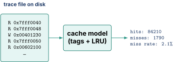
The appeal is real. It is fast, because there is no timing to compute, just tag lookups. It is perfectly reproducible, because the same trace gives the same answer every time, which matters enormously when you are comparing 40 configurations and need the difference between them to be the only variable. And it is easy to write, which is why it is a good first project.
2.4 The limitation that gets asked, and the two forms it takes
A trace was recorded on some other machine. That single fact produces two separate failures, and interviewers ask about both.
Failure one, no timing feedback. The trace is a fixed sequence. Nothing in the sequence responds to how fast your model runs. If your design has a slower L2, real software would experience different memory-level parallelism, different queue occupancies, different prefetcher training. The trace does not care. It replays the same addresses at the same relative positions no matter what your model does. Any effect where timing changes the sequence is invisible.
Failure two, no wrong path. This is the sharper one. A trace records what the program actually executed, which by definition is the correct path. A real out-of-order machine predicts branches, and when it predicts wrong it fetches, decodes, and often executes instructions on the wrong path before squashing them, as covered in Front End and Branch Prediction.
Those wrong-path instructions are not free. They issue loads that occupy MSHRs, they bring lines into the cache that the correct path may or may not want, they consume issue-queue entries and execution ports, and they occasionally prefetch something useful by accident. None of that is in the trace.
So here is the question you will get. "Why can a trace-driven simulator not properly evaluate a branch predictor change?" The answer is that a better predictor changes the set of wrong-path instructions, and the trace has no wrong-path instructions at all, so the mechanism you are trying to measure does not exist in the model. You can measure the misprediction rate from a trace, which is fine, but you cannot measure the performance effect of that rate change, because the cost of a misprediction depends on machine state the trace does not carry.
There is a subtler version. Trace-driven cache studies systematically report optimistic miss rates for one reason and pessimistic ones for another, and which dominates depends on the workload. Optimistic because no wrong-path pollution. Pessimistic because no wrong-path accidental prefetch. You cannot tell which without an execution-driven run, which rather defeats the purpose.
2.5 Execution-driven simulation
An execution-driven simulator actually interprets the program's instructions against a model of the machine. It has an architectural state, it fetches, it predicts, it executes down the wrong path, and it squashes. gem5's O3CPU is the standard open-source example and is the subject of Lab: gem5 Out-of-Order Modeling.
Because it executes, everything the trace could not model comes back. Timing feedback is captured, because the model's own timing determines what happens next. Speculation is modeled, because the model genuinely goes down the wrong path. Structural interactions are captured, because the queues in the model actually fill.
The price is speed. A detailed out-of-order model runs somewhere around 100,000 to 500,000 simulated instructions per second on a modern host. Call it 200 KIPS. A native machine at 3 GHz and IPC 2 executes 6 billion instructions per second. The slowdown is
That number drives Part 6 entirely. It is why you cannot simulate a full benchmark and why sampling is not optional.
There is a further split worth knowing. Cycle-approximate models get the structure right and the cycle counts within a few percent, which is plenty for comparing two designs. Cycle-accurate models claim to match the RTL cycle for cycle, which is far harder, much slower, and is the thing correlation in Part 7 tries to achieve. Most architecture exploration happens in cycle-approximate models, and treating a cycle-approximate number as an absolute prediction rather than a relative comparison is a classic mistake.
2.6 RTL simulation, and why it is not the answer to everything
RTL simulation is the ground truth for the design that exists. It captures everything, because it is the design.
It is also somewhere between and times slower than native, it requires the RTL to be written, and it requires the whole design to be integrated before you can measure a full-core number. Running SPEC on a full-core RTL model is not a thing anyone does. Instead you run short traces, tens of thousands to a few million cycles, chosen because they exercise the behavior you care about.
And RTL cannot answer the question that started this note, because the ROB size question must be settled before the RTL is written. That is the whole point of the hierarchy.
2.7 The rule
Use the cheapest model that can answer the question you are actually asking.
That sounds like a platitude until you apply it. Someone asks whether a 3-cycle L1 beats a 4-cycle L1 with a lower miss rate. Do not launch a 200-run gem5 campaign. Write the AMAT equation, get the answer in four seconds, and only escalate if the two options land within noise of each other. Someone asks how deep the store queue should be. That needs an execution-driven model, because store-queue occupancy depends on stall behavior which depends on timing. Someone asks whether the RTL's issue-queue wakeup logic is behaving as designed. That needs RTL, because no model above it contains the wakeup logic.
Escalating too early wastes months. Escalating too late produces a confidently wrong answer.
03.Part 3, structure sizing, worked properly
3.1 Why the ROB needs to be large, derived rather than asserted
Go back to Little's law from 2.2 and apply it to the real case.
A load misses all the way to DRAM. Say the latency is 200 cycles. Because the machine retires in order (see Out of Order Execution), that load sits at the head of the ROB for the whole 200 cycles and cannot retire. Every instruction that was fetched after it stays in the ROB too, because they cannot retire past it.
Meanwhile the machine is trying to keep working. If it can sustain 2 instructions per cycle on the independent work behind the miss, then over 200 cycles it wants to allocate
If the ROB holds only 128, it fills after 64 cycles and the machine stalls for the remaining 136 cycles of the miss. The ROB size directly caps how much of a memory latency you can hide.
That derivation gives you the shape of the answer before you run anything. It says the useful ROB size scales with (target IPC) times (the latency you want to cover). It also says the returns must eventually stop, because at some point you are covering the full DRAM latency and there is nothing more to cover.
3.2 The sweep
Now run it. In gem5 or an equivalent, hold everything else fixed and vary only the ROB, measuring IPC on a workload suite. Here is a representative sweep, with the marginal gain and the marginal gain per entry added computed alongside.
| ROB entries | IPC | IPC | Entries added | IPC per entry added |
|---|---|---|---|---|
| 32 | 1.31 | |||
| 48 | 1.54 | +0.23 | 16 | 0.0144 |
| 64 | 1.71 | +0.17 | 16 | 0.0106 |
| 96 | 1.90 | +0.19 | 32 | 0.0059 |
| 128 | 2.02 | +0.12 | 32 | 0.0038 |
| 192 | 2.13 | +0.11 | 64 | 0.0017 |
| 256 | 2.19 | +0.06 | 64 | 0.0009 |
| 384 | 2.23 | +0.04 | 128 | 0.0003 |
| 512 | 2.24 | +0.01 | 128 | 0.0001 |
Plot it and the shape is the point.
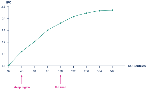
Three regions, and naming them is how you talk about this in an interview.
The steep region, 32 to 96. Every entry you add is doing work. The machine is window-limited, meaning it can see independent instructions but has nowhere to put them. Adding entries here is the cheapest performance in the design.
The knee, around 128 to 192. The curve bends. You are still gaining but the gain per entry has dropped by roughly 4x from the steep region.
The flat region, past 256. You are adding storage that is rarely occupied and, when it is occupied, contains instructions that cannot make progress anyway because they are dependent on the same stalled load.
3.3 Why it flattens, which is the actual question
Do not just say "diminishing returns." Say why, because there are three separate mechanisms and an interviewer is checking whether you know them.
One, the program runs out of independent work. A large window only helps if the instructions behind the stalled load are independent of it. Real programs have dependence chains. If instruction 200 past the miss depends on instruction 50 past the miss which depends on the miss itself, then a 512-entry ROB and a 128-entry ROB behave identically, because everything past entry 50 is blocked regardless. This is the intrinsic ILP limit of the program and no amount of hardware fixes it.
Two, some other structure binds first. The ROB is not the only queue. Sweep it alone and eventually the physical register file, the issue queue, the load queue, or the MSHR count becomes the binding constraint, at which point the ROB curve flattens for reasons that have nothing to do with the ROB.
This is why single-parameter sweeps mislead, and it is worth a table.
| ROB | PRF | Issue queue | Load queue | IPC | What is actually binding |
|---|---|---|---|---|---|
| 128 | 180 | 64 | 48 | 2.02 | ROB |
| 256 | 180 | 64 | 48 | 2.05 | PRF, ROB change bought almost nothing |
| 256 | 320 | 64 | 48 | 2.14 | issue queue |
| 256 | 320 | 96 | 48 | 2.19 | load queue |
| 256 | 320 | 96 | 72 | 2.27 | balanced |
Look at row two. Doubling the ROB from 128 to 256 bought 0.03 IPC, and a naive reading says the ROB does not matter. Row five shows it does, once the structures around it are scaled to match. The lesson is that structures must be sized as a set, and a sweep of one parameter with the others held at their old values will systematically underestimate its value. Balanced-design sweeps, where several structures scale together, are the honest version.
Three, the cost is not linear. A ROB entry is not just storage. The ROB is written by allocate, read by retire, searched by recovery, and its occupancy feeds stall logic. Doubling entries can push the structure out of a single cycle, which either costs a pipeline stage or costs frequency, and a 3 percent frequency loss to buy 1 percent IPC is a net loss.
3.4 Picking the design point
The engineering answer is not "where the curve flattens." It is where the marginal IPC stops justifying the marginal cost, and that requires a cost model alongside the performance model.
Suppose a ROB entry costs roughly 0.9 percent of the core area per 16 entries at the sizes involved, and suppose the team's rule of thumb is that a feature must return at least 1 percent performance per 1 percent area. Apply that to the sweep.
| Step | IPC | IPC percent | Approx area percent | Verdict |
|---|---|---|---|---|
| 64 to 96 | +0.19 | +11.1% | +1.8% | take it, easily |
| 96 to 128 | +0.12 | +6.3% | +1.8% | take it |
| 128 to 192 | +0.11 | +5.4% | +3.6% | take it |
| 192 to 256 | +0.06 | +2.8% | +3.6% | marginal |
| 256 to 384 | +0.04 | +1.8% | +7.2% | reject |
The design point is 192 or 256 depending on how much you value the marginal case, and the argument for it is now quantitative rather than aesthetic. That is what the whole exercise was for.
3.5 The other uses
Feature evaluation. Someone proposes a mechanism, say a stride prefetcher for the L2. Model it, measure IPC on the suite, and compare against the area and power estimate. The critical discipline is measuring across a suite, not one benchmark, because almost every prefetcher helps something and hurts something else. Report the geometric mean and the worst regression, and a feature with a 4 percent mean gain and a 9 percent worst-case regression is usually rejected, because shipped products cannot have workloads that get slower.
Bottleneck analysis. Where are the cycles going? Part 4 is entirely about doing this correctly.
Sensitivity analysis. How much does the conclusion depend on an assumption? If your ROB study assumed 200-cycle DRAM latency, rerun the key points at 150 and 250 and see whether the recommended size moves. Rerun with the branch predictor 1 percent better and 1 percent worse. If the recommendation is 192 entries at every assumption, you have a result. If the recommendation swings from 128 to 384 when DRAM latency moves by 25 percent, you do not have a result, you have an artifact of one assumption, and shipping a design based on it is how a chip arrives 10 percent slower than the model said.
04.Part 4, top-down analysis
4.1 The naive method, and watching it break
You have a slow program and you want to know why. The obvious approach is to count stall cycles by cause. Add a counter for cycles stalled on instruction-cache misses, one for data-cache misses, one for branch mispredictions, one for divider occupancy, and so on. Then look at which counter is biggest.
Watch this fail on a concrete case.
Take a 1000-cycle window. During it, an L2 miss is outstanding for 40 cycles. Overlapping with that, an instruction-cache miss is outstanding for 25 cycles, 20 of which fall inside the L2 miss window. A branch mispredict recovery takes 15 cycles, 10 of which also overlap the L2 miss. The machine was actually unable to make progress for 55 cycles total.
Now read the counters.
| Counter | Cycles reported |
|---|---|
| stalled on L2 miss | 40 |
| stalled on icache miss | 25 |
| stalled on branch recovery | 15 |
| naive sum | 80 |
| actual stalled cycles | 55 |
The counters sum to 80 for 55 real cycles, 145 percent of reality. Every overlapping cycle was counted twice or three times.
That is bad enough. The next failure is worse. Suppose you now fix the icache miss entirely, believing it was worth 25 cycles. The L2 miss is still there and still 40 cycles. You recover 5 cycles, not 25, because 20 of the 25 were hidden under the L2 miss and cost nothing. You optimized something whose measured cost was almost entirely fictional, which is exactly how weeks get spent for no gain.
The root problem is that in an out-of-order machine several things are in flight at once by design, and a cycle-based accounting has no way to decide which of the overlapping causes "owns" the cycle. Any assignment you invent is arbitrary.
4.2 The fix, count slots instead of cycles
Top-down microarchitecture analysis, introduced by Ahmad Yasin in a public 2014 paper and now implemented in the performance counters of essentially every modern high-performance core, fixes this by changing the unit of accounting.
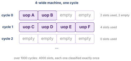
Instead of counting cycles, count pipeline slots. A pipeline slot is one opportunity to move one micro-operation through the machine's narrowest issue point, once, in one cycle. A 4-wide machine has 4 slots per cycle. Over 1000 cycles it has 4000 slots.
The crucial property is that a slot is a discrete thing that either got used or did not, and it has exactly one story. There is no overlap possible, because a slot is a single position in a single cycle. Ask of every slot what happened to it, and the answers partition perfectly.
4.3 The four buckets
Every slot goes through one decision tree, and it lands in exactly one of four buckets.
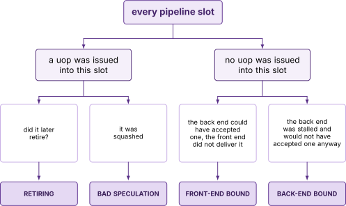
Retiring. The slot delivered a micro-operation that eventually retired and did useful architectural work. This is the good bucket, and its fraction is the machine's efficiency at that width.
Bad speculation. The slot delivered a micro-operation that was later thrown away. Dominated by branch mispredictions from Front End and Branch Prediction, with a smaller contribution from machine clears such as memory-ordering violations described in Load Store and Memory Ordering. Note that this bucket also implicitly charges for the recovery bubbles, because the empty slots during a pipeline flush are attributed here rather than to the front end, which is correct, since the front end was doing exactly what it was told.
Front-end bound. The slot was empty and the back end had room. The front end failed to supply. Causes are instruction-cache misses, iTLB misses, branch resteers, decode bandwidth limits, and fetch alignment.
Back-end bound. The slot was empty and the back end could not have taken anything anyway, because a resource was full or a dependency was unresolved. This is where cache misses, port contention, and dependence chains live.
The four sum to 100 percent by construction. That is not a happy accident, it is the entire design of the method.
4.4 Working real numbers
Take a 4-wide machine over a 1000-cycle window, so 4000 slots.
| Bucket | Slots | Fraction |
|---|---|---|
| Retiring | 1780 | 44.5% |
| Bad speculation | 320 | 8.0% |
| Front-end bound | 540 | 13.5% |
| Back-end bound | 1360 | 34.0% |
| Total | 4000 | 100.0% |
Sanity-check the retiring number against IPC. 1780 micro-operations retired over 1000 cycles is 1.78 uops per cycle, which on a 4-wide machine is 44.5 percent of peak. That matches the retiring fraction, as it must, and this cross-check is worth doing every time because it catches counter-configuration mistakes.
Now read the result. Back-end bound at 34 percent is the largest non-retiring bucket, so that is where the effort goes. Front-end bound at 13.5 percent is second. Bad speculation at 8 percent is real but is not the story.
Compare that to what the naive method would have told you. The naive counters, summing to more than 100 percent, would very likely have shown branch mispredictions as a large absolute number of cycles, because a 15-cycle penalty times a few thousand mispredicts is a big number, and a team could easily have spent a quarter on the predictor for a 2 percent return.
4.5 The drill-down
Each bucket subdivides, and the same partition property holds at every level. Here is the hierarchy.
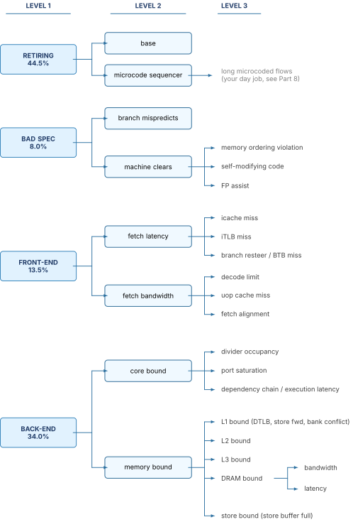
Drill the back-end bucket of the worked example and suppose it splits as follows.
| Level 2 | Slots | Percent of total |
|---|---|---|
| Core bound | 400 | 10.0% |
| Memory bound | 960 | 24.0% |
And memory bound splits again.
| Level 3 | Slots | Percent of total |
|---|---|---|
| L1 bound | 240 | 6.0% |
| L2 bound | 160 | 4.0% |
| L3 bound | 200 | 5.0% |
| DRAM bound | 360 | 9.0% |
Now you have an actionable answer. 9 percent of all issue slots are lost to DRAM. That is the single biggest identifiable cost, it is bigger than the entire bad-speculation bucket, and it points at prefetching, at the last-level cache, or at the memory controller. That conclusion could not have been reached from the naive counters, because the DRAM stalls would have been shadowed by everything overlapping them.
The workflow discipline is simple. Only drill into the largest bucket. Optimizing a level-3 leaf inside a level-1 bucket that is only 8 percent of slots caps your possible gain at 8 percent before you start.
4.6 How it maps onto real counters
The reason this method matters to a hardware engineer rather than only to a software performance analyst is that it is implemented in hardware counters, so the identical methodology runs on a model and on silicon.
The counters needed are few, and the formulas are arithmetic on them. Using the publicly documented event names as an illustration,
Read the last line carefully, because it is the honest part of the method. Back-end bound is computed as the residual, not measured directly. Counting "slots the back end refused" directly would require knowing, for every empty slot, whether the back end would have accepted a uop had one been offered, and that counterfactual is expensive to build in hardware. Taking it as the remainder is cheap and exact, given that the four buckets partition the space. The cost is that every measurement error in the other three lands in the back-end bucket, which is a real caveat and a good thing to know when someone shows you a top-down chart with 60 percent back-end bound.
The bad-speculation formula deserves the same attention. Issued minus retired counts the uops that were thrown away. The recovery term adds the slots that went empty during the flush, multiplied by the width because every slot in those cycles is lost. Without that second term you would undercount mispredictions badly, since the flush bubble is usually larger than the wrong-path work itself.
This counter mapping is the bridge to DFT and Silicon Debug. The same counters used for post-silicon performance analysis are part of the observability infrastructure that gets designed in, and if the counters are not there or are wrong, this entire method is unavailable on the shipped part.
05.Part 5, roofline
5.1 Arithmetic intensity, from an example
Top-down tells you where issue slots went inside a core. Roofline answers a different and coarser question. Is this code limited by how fast the machine computes, or by how fast it can move data?
The concept you need first is arithmetic intensity, and it is simpler than the name suggests. It is the number of useful arithmetic operations performed per byte moved between the processor and memory.
Work a real kernel. Vector add on double-precision values, c[i] = a[i] + b[i], for a large array that does not fit in cache.
Per element, count the arithmetic. One addition. That is 1 flop.
Per element, count the bytes. Read a[i], 8 bytes. Read b[i], 8 bytes. Write c[i], 8 bytes. That is 24 bytes.
Now a second kernel for contrast. Dense matrix multiply of two double matrices. The arithmetic is flops. With good cache blocking, the data moved is roughly the three matrices once each, bytes.
Two thousand times higher. That difference is the entire reason these two kernels behave completely differently on the same machine.
5.2 The roof
Now describe the machine with exactly two numbers. Peak compute, say 200 GFLOP/s. Peak memory bandwidth, say 100 GB/s.
Achievable performance is capped by both.
The first term is a horizontal ceiling. The second is a sloped ceiling, because if you only move bytes at 100 GB/s and each byte carries operations of work, you cannot exceed GFLOP/s no matter how fast the ALUs are.
The two ceilings cross at the ridge point, where , so
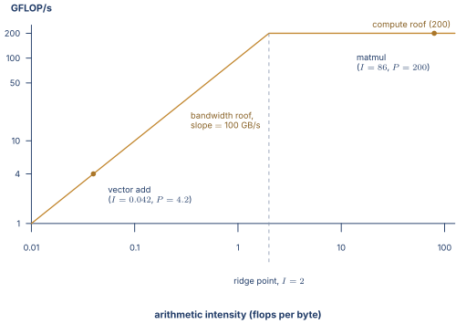
Place the two kernels. Vector add at is far left of the ridge, so its ceiling is GFLOP/s, which is 2.1 percent of the machine's peak compute. Matrix multiply at is far right of the ridge, so its ceiling is the full 200 GFLOP/s.
5.3 What that buys you
The conclusion is blunt and immediately actionable. For vector add, doubling the number of FPUs does nothing. Not a little, nothing. The kernel is at 2 percent of compute peak because bandwidth caps it, and adding compute moves a ceiling that was never binding. The only levers that help are ones that reduce bytes moved, such as fusing the loop with a neighbouring one so an array is not written and reread, using single precision to halve the bytes, or improving cache reuse to keep data on-chip.
For matrix multiply the opposite holds. Bandwidth upgrades are wasted and wider FMA units pay off directly.
That is the value proposition of roofline in one sentence. IPC tells you how well the machine is doing. Roofline tells you which resource to spend money on. A kernel running at 30 percent of peak compute sounds bad until you notice its arithmetic intensity puts its ceiling at 32 percent, at which point it is running at 94 percent of what is achievable and the engineer should go work on something else.
Real roofline plots add more ceilings. A lower horizontal line for scalar-only code without SIMD, another for code without FMA, and lower sloped lines for memory access patterns that do not achieve peak bandwidth such as strided or random access. Each ceiling you are stuck under names a specific optimization.
06.Part 6, workloads and the sampling problem
6.1 A conclusion is only as good as what you ran it on
Every number in Parts 3 through 5 came from running something. Change what you run and the numbers change, sometimes enough to reverse the design decision. This is where a great deal of performance work quietly goes wrong.
SPEC CPU is the industry-standard single-thread suite, split into integer and floating-point subsets, with run rules strict enough that published results are comparable across vendors. Its virtue is that it is well understood, widely reported, and hard to argue with. Its criticisms are real. It is compute-heavy relative to modern software, several of its components have small working sets by contemporary standards, and compilers have been tuned against it for decades so it partly measures compiler effort.
Consumer benchmarks such as GeekBench are what reviewers quote and therefore what customers see. They are short, which makes them sensitive to boost behavior and thermal state in ways that matter commercially and can mislead architecturally. A design tuned to win a 3-second burst benchmark is not necessarily the design that renders a web page fastest.
Real applications are what a company shipping consumer devices actually cares about. Browser page loads and JavaScript execution, video encode and decode, photo processing, compilation, application launch, UI responsiveness. These have properties SPEC does not, notably very large instruction footprints. A browser can have an instruction working set of several megabytes, which stresses the instruction cache and the branch predictor in ways no SPEC component does, and that is why front-end structures in Apple cores are as large as they are.
Microbenchmarks isolate exactly one behavior. A pointer-chase loop to measure load-to-use latency. A dependent-add chain to measure ALU latency. A wide independent stream to measure issue width. They are essential for characterization and for correlation in Part 7, because they produce a number you can predict analytically and therefore check. They are terrible for judging a design, because no real program looks like them and optimizing for them produces a machine that is fast at nothing anyone runs.
The discipline that follows is a suite, always, with the geometric mean reported alongside the per-workload spread and the worst regression called out explicitly.
6.2 Workload characterization
Before you can reason about why two workloads respond differently to a design change, you have to measure what they are.
| Property | What it is | What it drives |
|---|---|---|
| Instruction mix | fraction of loads, stores, branches, integer, FP, SIMD | port and unit counts |
| Branch density | branches per instruction | front-end width, predictor size |
| Branch predictability | misprediction rate with a given predictor | pipeline depth tolerance |
| Data working set | bytes touched repeatedly | cache capacities |
| Instruction footprint | distinct instruction bytes executed | icache and uop cache size |
| Memory-level parallelism | independent misses in flight at once | MSHR count, ROB size |
| Available ILP | independent instructions in a window | issue width, window size |
Now the point of the table. Two workloads with identical IPC can require completely different machines. Workload X runs at IPC 2.0 with 8 percent branches that are 99.5 percent predictable, a 200 KB working set that fits in L2, and long dependence chains. Workload Y also runs at IPC 2.0, with 24 percent branches at 96 percent predictable, a 40 MB working set, and abundant independent work. X wants deeper pipelining and more execution latency tolerance. Y wants a much better predictor, a much bigger last-level cache, and more MSHRs. Report only IPC and these two look interchangeable, which is why characterization exists.
6.3 Sampling, because full runs are impossible
Now confront the arithmetic from 2.5.
A single SPEC CPU component executes on the order of instructions on its reference input. At 200,000 simulated instructions per second,
That is one benchmark, one configuration. A suite of 20 benchmarks across the 9-point ROB sweep from Part 3 is runs, which is
Farms are parallel, so with 500 machines that is about ten days, but the sweep in 3.3 had four parameters, and you wanted sensitivity runs on top. The full-run approach does not survive contact with reality. You must sample.
The naive sample is to simulate the first billion instructions. This is badly wrong, because the first billion instructions of almost any program are initialization, which has nothing to do with the program's steady-state behavior. The second naive approach is to skip a fixed 10 billion and then sample, which is better and still arbitrary, because it happens to land wherever it lands.
6.4 SimPoint
SimPoint solves this properly, and the idea is worth understanding rather than name-dropping.
Programs execute in phases. A compiler spends a while in lexing, then in parsing, then in optimization, and each phase has a characteristic instruction mix, working set, and branch behavior. If you can identify the phases and how much time is spent in each, you can simulate one representative slice of each phase and weight the results.
The mechanism is the clever part. Chop the program's execution into intervals of, say, 100 million instructions. For each interval, record a basic block vector, which is simply a histogram counting how many times each static basic block in the program was executed during that interval, weighted by block length. That vector is a fingerprint of what code ran.
The insight is that intervals executing the same code in the same proportions behave the same way microarchitecturally, regardless of the actual data. So cluster the basic block vectors with k-means. Each cluster is a phase. Pick the interval nearest each cluster centroid as the representative, and weight it by the fraction of total intervals in that cluster.
Concretely, a program with 5000 intervals of 100 million instructions each, so 500 billion instructions total, might cluster into 10 phases.
| Simpoint | Cluster size | Weight | Interval simulated |
|---|---|---|---|
| 1 | 1450 intervals | 0.29 | 100M instructions |
| 2 | 980 | 0.196 | 100M |
| 3 | 720 | 0.144 | 100M |
| ... | ... | ... | ... |
| 10 | 85 | 0.017 | 100M |
| Total | 5000 | 1.000 | 1 billion |
Simulate 1 billion instructions instead of 500 billion, a 500x reduction, and estimate whole-program CPI as the weighted average
Published SimPoint accuracy on CPI is typically within a few percent of the full run, which is entirely good enough for the relative comparisons that Part 3 is doing. The 29-day run becomes about 90 minutes.
6.5 Warmup, which is where samples go wrong
Here is the part people underestimate, and it deserves numbers.
You have picked an interval 300 billion instructions into the program. You cannot execute the preceding 300 billion in detail, that was the whole point. So you fast-forward functionally, which means executing instructions for their architectural effect only, with no timing model, at maybe 100 million instructions per second, and then you switch to detailed mode and start measuring.
The problem is that at the moment you switch, your caches and predictors are empty. The real machine at that point in the program has warm caches, a trained branch predictor, a populated TLB, and a trained prefetcher. Yours has none of it.
Quantify it. Take a 100 million instruction sample with 20 percent loads, so 20 million memory accesses. Consider an 8 MB last-level cache with 64-byte lines, which holds
If the steady-state LLC miss count over that sample would have been about 60,000, then starting cold forces up to 131,072 additional compulsory misses as the cache fills. At a 200-cycle DRAM penalty that is
The sample at IPC 2.0 should take about 50 million cycles. You have added 26 million cycles of pure artifact, so the reported IPC is roughly
instead of 2.0. A 34 percent error, entirely from cold state, and it is not a random error, it is a systematic pessimism that will make every large-cache configuration look better than it is because the large cache takes longer to warm. Cold-start bias does not cancel out across configurations, it actively distorts the comparison you are running.
Branch predictors are worse in a different way. A TAGE predictor with tens of thousands of entries needs several million branches to reach steady-state accuracy. A sample that starts with a cleared predictor spends a meaningful fraction of its length training, reporting an inflated misprediction rate throughout.
Three standard defenses exist.
Functional warming. During fast-forward, do not just execute architecturally. Also feed every memory access to the cache models and every branch to the predictor models, updating their state without computing any timing. It is slower than pure fast-forward but far faster than detailed simulation, and it arrives at the sample with genuinely warm structures.
Checkpointing. Save the complete state at the sample boundary once, including architectural state and cache tags, predictor tables, TLB contents, and prefetcher state. Every subsequent run restores from the checkpoint instantly. This is what makes a 180-run sweep tractable, since the expensive warm-up is paid once rather than 180 times. The catch is that a checkpoint of microarchitectural state is only valid for the configuration it was taken on, so a ROB sweep can share checkpoints but a cache-size sweep cannot.
Detailed warming. Run detailed simulation for some millions of instructions before the measurement window opens and discard those results. Simple, correct, and expensive.
The rule to carry into an interview is short. A sample with cold state does not report a slightly wrong answer, it reports a meaningless one, and the error is biased rather than random.
07.Part 7, correlation
7.1 What it is and why it is the design engineer's half
The model said the core would run SPECint at IPC 2.19. The RTL exists now. Someone runs a trace through both and the RTL reports 2.02.
That gap is 8 percent. It is far too large to ignore, and somebody has to find out where it went. That is correlation, and it is where an RTL engineer contributes to performance work, because finding the answer means reading RTL, reading waveforms, and reasoning about what the logic actually does cycle by cycle. Architecture background helps. RTL debugging skill is what closes it.
7.2 The method
Correlation is a discipline, not an act of inspiration.
One, run identical stimulus. Same instruction sequence, same starting state, same memory contents. This sounds trivial and is the most common source of false discrepancies, because the model and the RTL testbench usually have completely different mechanisms for loading a program and initializing memory.
Two, compare aggregate cycle count first. If the total matches within a fraction of a percent, you are done for that test. If it does not, you have a number to chase.
Three, compare event counts, not just cycles. Instructions retired, branch mispredicts, L1 misses, L2 misses, stall cycles by source, structure full events, port utilizations. This localizes the discrepancy without any waveform work. If cycles differ by 8 percent but every event count matches, the difference is in latency or arbitration rather than in behavior. If the L2 miss counts differ by 40 percent, you have your answer's neighbourhood.
Four, compare per-instruction retire timestamps. This is the sharpest tool. Emit, from both the model and the RTL, a record of the cycle at which each instruction retired. Then diff them and find the first instruction where the two diverge.
| instr # PC model retire RTL retire delta | |
| ------- ---------- ------------ ---------- ----- | |
| 44 0x1000a4c 118 118 0 | |
| 45 0x1000a50 118 118 0 | |
| 46 0x1000a54 119 119 0 | |
| 47 0x1000a58 119 127 +8 <-- first divergence | |
| 48 0x1000a5c 120 128 +8 | |
| 49 0x1000a60 121 129 +8 | |
| ... | |
| 412 0x1000f10 1004 1012 +8 | |
| 413 0x1000f14 1006 1021 +15 <-- second event |
The first divergence at instruction 47 is where you start. Everything after it inherits the offset and is not independent evidence. Look at instruction 47, see what it is, and see what the RTL waveform shows it waiting for that the model did not model. The second jump at instruction 413 is a genuinely separate event, and correlation work proceeds one divergence at a time.
7.3 The three categories of discrepancy
Every gap you find falls into exactly one of three categories, and classifying it correctly is most of the value, because the three have completely different owners and completely different fixes.
Category one, the model is wrong. The model idealized something the RTL cannot do. This is the most common outcome and it is not a failure of the modeling team, it is inherent, because a model that captured everything would be the RTL. Typical cases include a structural conflict the model did not represent, such as two operations sharing a write port that the model gave separate ports. An arbitration policy the model treated as fair when the RTL implements fixed priority, as in Arbiters FIFOs and CAMs. A pipeline depth that grew by a stage during implementation because a path would not close timing. A latency the model set to 4 that the RTL implements as 5. A bypass network the model assumed was full when the RTL omitted a rarely used path to save area.
The fix is to update the model, and the important consequence is that every performance projection made with the old model is now suspect and may need rerunning. Finding a model error late in a project is genuinely expensive for that reason.
Category two, the RTL is wrong. There is a defect. It may be a functional bug that verification missed, but far more often it is a performance defect, meaning the RTL computes correct results and does so more slowly than the design intended. Section 7.4 is about these.
Category three, both are right and the comparison is unfair. The two runs were not actually comparable. Different warmup state. Different memory initialization. Different definitions of when the cycle counter starts and stops. One counting micro-operations and the other counting architectural instructions. A model measuring from reset and RTL measuring from the first fetch after boot code. This category is embarrassing and extremely common, and it is why the first hour of any correlation effort should be spent proving the two runs are comparable at all.
Here is the classification workflow as a decision aid.
| Symptom | Most likely category | First thing to check |
|---|---|---|
| Constant offset from cycle zero | unfair comparison | counter start conditions, reset handling |
| Event counts identical, cycles differ uniformly | model wrong | a latency or pipeline depth constant |
| One event count differs wildly | model or RTL | which structure that event belongs to |
| Divergence starts at one instruction and stays constant | either | what that instruction waited on in RTL |
| RTL matches on microbenchmarks, differs on real code | model wrong | an interaction the microbenchmark does not create |
| RTL slower only under high occupancy | RTL wrong | queue full logic, credit accounting |
That last row is worth remembering, because it is the classic signature of the most common class of performance bug.
7.4 Performance bugs, and why verification does not find them
This is the concept in this note that most cleanly separates a candidate who has been near real silicon from one who has not.
A performance bug is a defect that produces correct results slowly.
Sit with what that means for verification. Everything in Verification Methodology is built on comparing the design's output against a reference. Scoreboards check values. Assertions check protocols. Formal proves properties. Coverage measures whether scenarios were exercised. Every one of those mechanisms passes on a design that is functionally perfect and 15 percent slow, because the answers are right. The scoreboard has nothing to complain about. The chip works.
Concrete examples, each of which has really happened somewhere.
A queue is specified as 16 entries, and an off-by-one in the full-detection logic asserts full at 15. Functionally flawless, because backpressure works correctly. You have silently paid for a 16-entry structure and deployed a 15-entry one, and if the structure is near a knee in its sizing curve you have given up real performance.
A bypass path from a specific execution unit back to a specific operand input was omitted, so those dependent operations take the register-file route and cost two extra cycles. Correct results, always. A latency penalty on a dependence pattern that may be common.
A stall condition is written more conservatively than the specification requires, stalling on any outstanding operation rather than on a genuine conflict. Correct, and needlessly serializing.
A clock-gating enable is too aggressive and a unit takes an extra cycle to wake, which shows up only as a small latency adder on the first operation after an idle period. Correct, and a real cost on bursty workloads. This one connects directly to Power Fundamentals and Clock Gating and is exactly the class of defect a gating-efficiency push can introduce.
A prefetcher's training logic has a condition inverted so it trains on the wrong events. It still issues legal prefetches, they are just useless. Correct, and you built a useless prefetcher.
Correlation is the only systematic defense against all of these. There is no other stage in the flow that would catch them. And they are expensive to find late, because the fix may be structural, which means an RTL change deep in a block that has already been through timing closure and physical design, which means the fix costs schedule as well as engineering.
There is a related discipline worth mentioning, which is writing performance assertions alongside functional ones. An assertion that fires when a queue's occupancy never exceeds 15 over a long run, or when a specific bypass is never exercised, or when a stall signal asserts under conditions that should not stall, catches the whole class above during ordinary regression rather than during correlation. This is where the formal-property skill from power-management verification transfers directly.
7.5 Post-silicon correlation
The loop closes on real hardware.
Once parts come back, run the same workloads on silicon and read the performance counters, which are the hardware event counters described in DFT and Silicon Debug. Compute the top-down breakdown from Part 4 on silicon, and compare it to the top-down breakdown from the model and from RTL simulation. Because the methodology is identical across all three, the comparison is apples to apples.
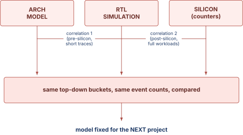
Post-silicon correlation does three things at once. It validates the RTL against real workloads that were far too long to simulate, so behaviors that only appear after billions of instructions finally get exercised. It validates the model against reality, which is what makes the model trustworthy for the next project. And it finds the performance bugs that survived everything, which then get characterized, worked around in firmware or the compiler if possible, and fixed in the next stepping.
The organizational point is that a model is only as credible as its last correlation. A team that skips post-silicon correlation is designing the next chip with a model nobody has checked, and the errors compound.
08.Part 9, check yourself
Answer out loud, in full sentences, as if an interviewer asked. If you cannot, reread the section named.
- Write the iron law of performance and explain why Apple buys performance through IPC rather than frequency. (1.3)
- Rank analytical, trace-driven, execution-driven, and RTL models by speed and accuracy, and say what each cannot capture. (2.1 through 2.6)
- An engineer proposes a bigger L1 with one extra cycle of hit latency. How do you evaluate that in under a minute? (2.2)
- State Little's law, give a non-hardware example, and use it to argue for a ROB size. (2.2, 3.1)
- Why can a trace-driven simulator not properly evaluate a branch predictor change? Give both reasons. (2.4)
- You sweep ROB size and IPC barely moves past 128. Give three distinct explanations and say how you would tell them apart. (3.3)
- Why does sweeping one structure with the others held fixed systematically understate its value? (3.3)
- Show with numbers how naive stall attribution can sum to more than 100 percent, and why that leads to wasted optimization effort. (4.1)
- Why does top-down count slots rather than cycles, and why does that guarantee the buckets partition? (4.2, 4.3)
- Name the four top-down buckets, say what each means, and explain why back-end bound is computed as a residual. (4.3, 4.6)
- Compute the arithmetic intensity of a double-precision vector add and say what it implies about adding FPUs. (5.1, 5.3)
- A kernel runs at 30 percent of the machine's peak FLOP rate. Is that bad? What do you need to know first? (5.2, 5.3)
- Why is simulating the first billion instructions of a benchmark a bad sample, and how does SimPoint choose better? (6.3, 6.4)
- Quantify what happens to reported IPC if you start a 100 million instruction sample with a cold 8 MB last-level cache. (6.5)
- Your RTL reports 8 percent lower IPC than the model on the same trace. Walk through your correlation method step by step. (7.2)
- Give the three categories of model-versus-RTL discrepancy and one concrete example of each. (7.3)
- What is a performance bug, why does functional verification never catch one, and name three concrete examples. (7.4)
- How would you use hardware performance counters to correlate silicon against the model, and what does that buy the next project? (7.5)
09.Part 10, related notes
- Lab: gem5 Out-of-Order Modeling to actually run the sweeps in Part 3, which is the single highest-value thing you can do for this topic
- Out of Order Execution for the ROB, issue queue, and physical register file that Part 3 is sizing
- Front End and Branch Prediction for the mispredictions that fill the bad-speculation bucket and for why traces cannot model them
- Cache Organization and Prefetching for AMAT, MSHRs, and the memory-level parallelism that sets the memory-bound bucket
- Load Store and Memory Ordering for the memory-ordering machine clears inside bad speculation
- DFT and Silicon Debug for the performance counters that make post-silicon correlation possible at all
- Verification Methodology for the scoreboards and assertions that pass cleanly on a slow chip, which is the whole reason correlation exists
- Power Fundamentals and Clock Gating for the wakeup-latency class of performance bug and your own strongest hook into this material
- Project: A Trace-Driven Cache Simulator in C++ for building the trace-driven model whose limits Part 2 describes
- Trends, Constraints, and Quantitative Principles for Amdahl's law and why the geometric mean is the right average for a benchmark suite