Verification Methodology

July 31, 2026·44 min read·advanced

You have built an 8-bit adder, a block taking two 8-bit numbers plus a carry-in. You want to know whether it is correct. Not "probably correct." Correct.

01.Part 1, the problem verification exists to solve

1.1 Test something small exhaustively, then watch it stop working

You have built an 8-bit adder, a block taking two 8-bit numbers plus a carry-in. You want to know whether it is correct. Not "probably correct." Correct.

There is an obvious way. Try every input. There are $2^8$ values for $A$ , $2^8$ for $B$ , and 2 for the carry-in.

$2^8 \times 2^8 \times 2^1 = 2^{17} = 131{,}072$

A simulator doing a million vectors per second finishes in 0.13 seconds. When it reports no mismatches you are not guessing. Every input the adder will ever see has been checked, so no untested case remains to hide a bug in. That is what complete verification looks like, and this is the only place in the note you will see it.

Widen to 16 bits and the count is $2^{33} \approx 8.6$ billion, about 2.4 hours. Doable overnight. Widen to 32 bits and it is $2^{65} \approx 3.7 \times 10^{19}$ , which is 1,170 years even at a billion vectors a second. Widen to 64 bits, which is what a real CPU adder is, and it is $2^{129} \approx 6.8 \times 10^{38}$ , or $2.2 \times 10^{22}$ years. The universe is about $1.4 \times 10^{10}$ years old.

Adder width	Input combinations	Time at $10^9$ vectors per second
8 bits	$1.3 \times 10^5$	0.13 ms
16 bits	$8.6 \times 10^9$	8.6 seconds
32 bits	$3.7 \times 10^{19}$	1,170 years
64 bits	$6.8 \times 10^{38}$	$2.2 \times 10^{22}$ years

Nothing changed conceptually between the first row and the last. Same logic, same structure, same material as Arithmetic Hardware. One parameter changed and complete verification went from trivial to physically impossible.

1.2 Now add state

That adder was combinational, so an input fully determines an output. Real blocks have flops, and a flop remembers. A block with $n$ flops has $2^n$ states, so what you must cover is inputs crossed with states crossed with the input sequences that reach those states.

Take $n = 100$ , a small block. A 32-bit register, a few counters, and a small FSM get you there. $2^{100} \approx 1.27 \times 10^{30}$ , which at a billion states per second is $4.0 \times 10^{13}$ years, roughly 2,900 times the age of the universe. The Resource Controller IP you built at Intel has more than 100 flops in its status registers alone, and a modern CPU core has around a hundred thousand state bits, whose state count written in decimal has 30,103 digits.

1.3 Reachable states, and why they only sometimes save you

Most of those $2^n$ encodings are unreachable, meaning no legal input sequence from reset ever produces them. An FSM with 8 states encoded one-hot, one flop per state with exactly one high, has 8 flops and $2^8 = 256$ encodings but only 8 reachable states, since the other 248 have two flops high or none. That is a factor of 32 from noticing nothing more than which states exist, and it is exactly what a formal tool computes for you in 5.2.

Do not oversell it. A 64-entry FIFO of 32-bit data has 2048 storage bits and essentially all of those contents are reachable, since you can write any data into any entry. Reachability saved you nothing. That is the honest reason formal is strong on control and weak on datapaths, which returns in 5.6.

1.4 Two families, different in kind

Simulation picks specific inputs, runs them, checks specific outputs. It scales to any design size. What it proves is exactly this. The design behaved correctly on the vectors you ran. Run ten billion cycles on that 100-flop block and you have visited at most one state in $10^{20}$ . Confidence rose. Coverage of the space did not meaningfully move.

Formal runs no vectors. It takes a property, a mathematical statement about behavior, and either proves it holds for every legal input sequence or produces a sequence that violates it. When formal says a property holds, no input sequence breaks it. The price is that it scales terribly and on a large block simply runs out of memory.

	Simulation	Formal
What it examines	the vectors you supplied	all legal input sequences
Scales to	any design size	hundreds to a few thousand state bits
Passing means	"no bug on these vectors"	"no bug exists, within the property's scope"
Failing gives	a failing waveform	a minimal counterexample waveform
Cannot finish means	you ran out of patience	inconclusive, no information either way
Needs stimulus	yes, and writing it is most of the work	no
Main failure mode	you never thought of the case	you over-constrained and proved nothing

The judgment tested in an interview is not which is better. It is which you reach for on a given block, and that comes from 5.6.

02.Part 2, simulation-based verification

2.1 What a testbench is, and the four jobs

A testbench is ordinary code that is not part of the chip. It instantiates the design, universally the DUT for design under test, drives its inputs, watches its outputs, and complains when something is wrong. It can use every software feature the language offers, none of it synthesizable and none of it needing to be.

Every testbench, from twenty lines to a hundred thousand, does four jobs. Generate stimulus, deciding what inputs to apply. Drive, turning that into pin activity that respects the protocol. Observe, watching what the DUT did. Check, deciding whether it was right. Almost every methodology debate is about organizing those four so they can be reused and so the checking is trustworthy, and the UVM component names in Part 3 map onto them almost one to one.

2.2 Directed tests, and where they run out

A directed test is one test per feature with exact stimulus and exact expected results. For an 8-entry FIFO you push 8 and check full, pop 8 and check empty, then write another for simultaneous push and pop and another for reset mid-transaction. They are easy to read, easy to debug, and they map one to one onto a specification document, which makes review straightforward. Every project's early bring-up is directed testing.

The ceiling is exact. A directed test finds bugs in cases the author thought of. The author thought of full, empty, simultaneous, and reset. The author did not think of "push when the read pointer has just wrapped and a reset arrives in the same cycle the almost-full threshold is being reprogrammed." Bugs cluster in the cases nobody enumerated, precisely because the cases people enumerate are the ones the designer also enumerated and therefore handled. There is an arithmetic problem too. Six independent configuration bits give 64 configurations, and twenty scenarios each is 1,280 tests. Nobody writes those by hand.

2.3 Constrained random, with the numbers worked

Constrained random verification inverts it. You describe the legal space of stimulus with constraints and let the tool generate randomly inside it, so the machine explores combinations no human would write down.

Code

class Transaction;
    rand bit [31:0] addr;
    rand bit [3:0]  len;        // beats in the burst, 0 encodes 1 beat
    rand bit        is_write;
    rand bit [2:0]  size;       // log2 of bytes per beat
    constraint legal_addr {     // word aligned, 256 MB aperture
        addr[1:0] == 2'b00;
        addr < 32'h1000_0000;
    }
    constraint legal_size { size inside {0, 1, 2}; }
    // Bias toward short bursts without making long ones impossible.
    constraint len_dist { len dist { 0 := 30, [1:7] := 50, [8:15] := 20 }; }
endclass
```text
Read `constraint` as a statement of what is legal, not of what will happen. The solver picks a random assignment satisfying every constraint at once. `dist` biases probabilities without forbidding anything, which is the important detail, since weight 20 on long bursts makes them less likely rather than impossible.
Now make it concrete. The bug you are hunting lives in a **16-beat write burst that crosses a 4 KB page boundary**. A 16-beat burst of 4-byte beats spans 64 bytes, and a 4 KB page holds 1,024 word slots, so the burst crosses if the starting word index is 1,009 or higher, which is 15 of 1,024 slots and $P_{\text{cross}} = 0.0146$. Sixteen beats means `len == 15`, probability $0.20 \times \tfrac{1}{8} = 0.025$ under that `dist`. And `is_write` is a fair coin.
$$P_{\text{hit}} = 0.0146 \times 0.025 \times 0.5 = 1.83 \times 10^{-4}$$
About **one transaction in 5,500**. How many for 95 percent confidence of at least one hit? The probability of missing $n$ times is $(1-p)^n$, and you want that under 0.05.
$$n = \frac{\ln 0.05}{\ln(1 - 1.83\times10^{-4})} \approx \frac{-3.00}{-1.83\times10^{-4}} \approx 16{,}400$$
A rule worth memorizing falls out. **To be about 95 percent sure of hitting a one-in-$N$ event, run about $3N$ trials.** Sixteen thousand transactions is a few minutes, so random finds this bug easily and nobody had to think of it.
Make it harder. Suppose it only fires when that page-crossing write happens **while the response FIFO is nearly full**, true on maybe 1 cycle in 64. Now $p = 2.9 \times 10^{-6}$ and you need about **1.05 million** transactions. Stack two more such conditions and you are into billions, and pure randomness never finds it.
That is the honest limit, and it is why the next two parts exist. You need **coverage** to tell you the case was never hit, then a **biased constraint or a directed test** to force it. Random stimulus without coverage measurement is not verification, it is activity.
### 2.4 Scoreboards, and why the reference model must be independent
Generating a million random transactions is easy. Deciding whether the DUT responded correctly to a million of them is the actual problem, because nobody inspects a million waveforms. The answer is a **reference model**, also called a golden model or predictor, which computes what the DUT **should** have done, plus a **scoreboard**, which compares should against did.
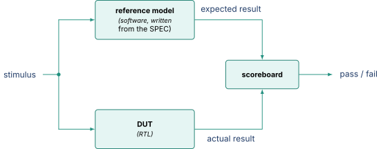
<Figure src="/figures/hardware-interview-prep/iv-19-Verification-Methodology-fig01.svg" alt="The same stimulus travels two independent paths and the scoreboard compares where they land, so the comparison has power only over the parts of the two paths that genuinely differ." caption="The same stimulus travels two independent paths and the scoreboard compares where they land, so the comparison has power only over the parts of the two paths that genuinely differ." id="fig:19-Verification-Methodology-1" />
The model does not have to be cycle accurate and usually should not be. For a memory bus it is an associative array, `bit [31:0] mem [bit [31:0]]`, where a write stores and a read looks up. It models **what** the design computes, not **how** or **when**, and timing is checked separately by interface assertions from [RTL Design and SystemVerilog](/learn/hardware-interview-prep/rtl-design-and-systemverilog). Real scoreboards are queues keyed by transaction ID rather than a same-cycle compare, because the DUT may reorder responses.
Now the "why" question, which usually gets too shallow an answer. The shallow answer is "so it does not have the same bugs." The full answer is about **where a bug can hide**. Verification produces two answers to the same question through two paths and compares them. If the paths share a step, a mistake in that shared step produces the same wrong answer twice and the comparison passes. **The comparison has power only over the parts of the two paths that genuinely differ.**
So suppose the model is written by reading the RTL. The specification says a page-crossing burst must be split. The designer misread it and did not split. The verification engineer opens the RTL, sees no splitting, and writes a model that does not split. The scoreboard compares "no split" against "no split" and reports pass. **The bug is now invisible and stamped as verified**, which is worse than not testing it, because you believe something false.
Three rules follow. Write the model from the **specification**, not the RTL. Have a **different person** write it where the block justifies the cost. And when the scoreboard mismatches, **do not assume the RTL is wrong**, because on a healthy project the model is wrong roughly a third of the time, and about a tenth of the time both are right and the specification is ambiguous. That last case is the most valuable finding of all, since an ambiguous spec will be read differently by the software team.
---
## Part 3, UVM
### 3.1 The problem it was invented to solve
Suppose every engineer builds their testbench their own way. Block A drives its interface with tasks in a module, block B uses a class with a queue, block C uses a program block. All three work. Now integrate the three and try to reuse their testbenches. You cannot, because there is no common shape to plug together, so you write a fourth from scratch and the block-level tests that took nine months are thrown away. Then buy an AXI verification IP and it arrives in the vendor's own shape, plugging into nothing.
**UVM**, the Universal Verification Methodology, is an IEEE-standardized SystemVerilog class library that solves this by dictating the shape. It names what a component that drives pins is, what a component that watches pins is, how they connect, how they are configured, and how they are built. It is a standard, not a technology. Nothing in UVM is impossible without it. The value is that everyone does it the same way.
### 3.2 The components, one at a time
**Sequence item.** The transaction object. The `Transaction` class from 2.3 is one, extending `uvm_sequence_item`.
**Sequence.** A generator of items describing a scenario at the transaction level, for example "10 random writes, then read back the same 10 addresses." Sequences call other sequences, which composes complicated scenarios from simple pieces. This is the **generate** job.
**Sequencer.** The traffic controller between sequences and the driver, doing arbitration when several sequences want the same interface and handing one item at a time to the driver on request. You rarely write a custom one.
**Driver.** Converts an item into pin wiggles obeying the protocol, spending however many cycles that takes. This is the **drive** job, and it is the only component that writes DUT inputs.
**Monitor.** Watches the pins and reconstructs transactions from them, entirely **passive**, driving nothing. This is the **observe** job. Its most important property is that it must be written **independently of the driver** and must never peek at the driver's state, for exactly the reason in 2.4. If the monitor asks the driver what it sent, a driver bug becomes invisible. It reconstructs from the wires alone, the way an oscilloscope would.
**Agent.** A container bundling sequencer, driver, and monitor for one interface plus its configuration. An agent is **active**, meaning it drives, or **passive**, meaning only the monitor is built. That switch is why agents reuse upward. A block-level active agent becomes passive at SoC level, where real traffic comes from a neighboring block, and the same monitor keeps checking the protocol.
**Scoreboard.** Receives transactions from monitors and decides pass or fail, usually holding or calling the reference model. This is the **check** job.
**Coverage collector.** Receives the same transactions and samples covergroups, which is Part 4.
**Environment.** Holds agents, scoreboard, coverage, and sub-environments. Environments nest, so a subsystem environment contains three block environments.
**Test.** The top-level class. It builds the environment, applies configuration, and starts sequences. A "test" in the regression list is one of these. Different tests reuse the same environment and differ only in configuration and sequences, which is why adding the 400th test to a mature environment is a twenty-line job.
**Config object and config database.** A plain object of knobs published into a global lookup, so a component four levels deep retrieves its settings without every intermediate level passing them down.
### 3.3 The whole thing in one picture
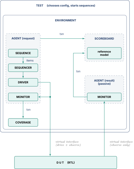
<Figure src="/figures/hardware-interview-prep/iv-19-Verification-Methodology-fig02.svg" alt="The test builds the environment, the request agent turns sequence items into pin activity, and the monitors reach the scoreboard from the wires alone rather than from anything the driver tells them." caption="The test builds the environment, the request agent turns sequence items into pin activity, and the monitors reach the scoreboard from the wires alone rather than from anything the driver tells them." id="fig:19-Verification-Methodology-2" />
Trace one transaction. The test starts a sequence, which creates an item and hands it to the sequencer, which gives it to the driver when the driver is free. The driver spends four clock cycles putting it on the wires. The request monitor, watching those same wires with no knowledge of the driver, reconstructs an equivalent transaction and broadcasts it to the scoreboard and the coverage collector. The scoreboard feeds it to the reference model and stores the expected response. Cycles later the DUT responds, the result monitor reconstructs the response, and the scoreboard pops the expected value and compares.
### 3.4 What standardization buys, and when to skip it
Three distinct kinds of value. **Vertical reuse**, where a block-level agent is instantiated unchanged at subsystem and SoC level flipped to passive, so its protocol assertions and coverage keep running and catch integration-created violations with the same code. **Horizontal reuse**, where third-party VIP for AXI, PCIe, or LPDDR arrives as UVM agents and integration is instantiation rather than adaptation. **Team scaling**, where twenty engineers work on one testbench because the structure is not a matter of opinion.
An interviewer asking about UVM is often probing whether you apply it reflexively, so say plainly that it is not always right. The library is large, phasing is subtle, the config database is a global namespace with the debugging pain that implies, and a testbench that would be thirty direct lines becomes several hundred. Four cases where plain SystemVerilog wins. A **small leaf block** with one simple interface that will never be reused. **Formal-first blocks**, where the plan is properties rather than vectors and you need only smoke tests. **Bring-up work**, where the question is "does this basically move." And **C or C++ processor verification flows**, where the reference model is an instruction set simulator and the stimulus is compiled programs, so UVM appears only around the bus interfaces. UVM is infrastructure for reuse, and with no reuse you pay the cost and collect no benefit.
---
## Part 4, coverage
### 4.1 Code coverage, automatic and weak
**Code coverage** is measured by the simulator with no work beyond a compile switch, and it reports which parts of the source the simulation touched. **Line** coverage asks whether a line executed. **Branch** coverage asks whether each `if` went both ways and each `case` arm occurred. **Condition** coverage asks, for `if (a && b)`, whether each operand independently took both values, which branch coverage does not, since `a=1,b=1` and `a=0,b=0` satisfy branch coverage without ever distinguishing which operand caused the false. **Toggle** coverage asks whether each signal bit went both directions, and it is the one that finds tied-off buses and unconnected ports. **FSM** coverage asks whether all states were visited and all legal transitions taken, and the transition half is the useful half, since a 6-state FSM might have 20 legal transitions.
It is necessary and it is weak, which is easy to demonstrate.
```systemverilog
always_comb begin
    if (push && !full)      next_count = count + 1;
    else if (pop && !empty) next_count = count - 1;
    else                    next_count = count;
end
```text
A test that pushes once, pops once, and idles once achieves **100 percent line and branch coverage** here. Every line ran, every branch went both ways. And you have not tested pushing when full, popping when empty, or simultaneous push and pop, which is where the bug is.
One line for an interview. **Code coverage measures what the tests touched. It cannot measure what the tests meant, and it cannot see a feature that was never implemented at all**, because there is no source line to leave uncovered.
### 4.2 Functional coverage, hand-written and meaningful
**Functional coverage** is written by a human who read the specification, and it measures whether the interesting **scenarios** occurred, in terms of the design's intent rather than its source text. A **covergroup** holds **coverpoints** which hold **bins**. A coverpoint watches an expression, a bin is a named set of values you care about, and coverage is the fraction of bins hit.
```systemverilog
covergroup bus_cg @(posedge clk);
    option.per_instance = 1;
    len_cp: coverpoint txn.len {
        bins single = {0};
        bins short  = {[1:3]};
        bins medium = {[4:7]};
        bins long   = {[8:15]};
    }
    kind_cp: coverpoint txn.is_write {
        bins read  = {0};
        bins write = {1};
    }
    align_cp: coverpoint page_cross {
        bins inside_page = {0};
        bins crosses     = {1};
    }
endgroup
```text
That is $4 + 2 + 2 = 8$ bins. Note what you did that a tool cannot. You decided a length of 4 and a length of 7 are the same case, and that a length of 0 is special enough for its own bin. That judgment is the content, and no tool can know a single-beat burst exercises a different path than a 3-beat one.
### 4.3 The cross, and exactly what it catches
The answer here is not obvious until worked. Run a regression that produces these three kinds of traffic and nothing else.
| Scenario | count | `len_cp` bin | `kind_cp` bin |
|---|---|---|---|
| short reads | 40,000 | short | read |
| short writes | 35,000 | short | write |
| long reads | 25,000 | long | read |
Score the coverpoints individually. `len_cp` needed `short` and `long`, both hit. `kind_cp` needed `read` and `write`, both hit. On the two coverpoints that matter, **you are at 100 percent**. The report is green and you would ship. And you never performed a single **long write**, which is the transaction that fills the write data buffer and is the one most likely to expose a flow-control bug.
Add one line.
```systemverilog
    lk_cross: cross len_cp, kind_cp;
```text
The cross creates a bin per combination, so $4 \times 2 = 8$. You hit short-read, short-write, and long-read. That is 3 of 8, **37.5 percent**, and the report names `long`&`write` in the hole list explicitly.
The principle in one sentence. **Individual coverpoints tell you each variable took its interesting values. A cross tells you they took them at the same time, and bugs live in the combinations.**
Cross bins also multiply. Adding `align_cp` gives $4 \times 2 \times 2 = 16$, and a fourth coverpoint with 5 bins gives 80, most of them uninteresting or illegal.
```systemverilog
    full_cross: cross len_cp, kind_cp, align_cp {
        // A single-beat access can never cross a page boundary.
        illegal_bins impossible = binsof(len_cp.single) && binsof(align_cp.crosses);
        // Read alignment is not part of this feature's plan.
        ignore_bins  dont_care  = binsof(kind_cp.read)  && binsof(align_cp.crosses);
    }
```text
`illegal_bins` means "if this ever happens, fail the test," because it is a stimulus bug. `ignore_bins` means "this cannot happen or does not matter, remove it from the denominator." The difference matters, because an `ignore_bins` written to make a number go up is exactly how a coverage report becomes a lie.
### 4.4 Closure and signoff
**Coverage closure** is the loop that occupies the last third of a project.
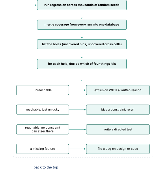
<Figure src="/figures/hardware-interview-prep/iv-19-Verification-Methodology-fig03.svg" alt="Closure is a loop rather than a report, and its work is the decision made about each hole, one of only four things a hole can turn out to be." caption="Closure is a loop rather than a report, and its work is the decision made about each hole, one of only four things a hole can turn out to be." id="fig:19-Verification-Methodology-3" />
**Merging is what makes it work**, since no single seed covers much, and a thousand seeds each covering 20 percent might merge to 85 percent. The database merges across runs, across tests, and often across simulation and formal, because a formally proven property can legitimately close a hole.
**The signoff criteria are agreed in advance and written down.** Typically 100 percent of the functional coverage plan, since the plan is a negotiated document rather than everything conceivable, plus code coverage above a threshold such as 98 percent line and branch, plus zero unexplained exclusions, plus all assertions passing **with no assertion having zero hits**, plus the regression clean on every seed for some number of consecutive nights.
That assertion criterion deserves emphasis. **An assertion that never fired is not evidence of correctness, it is evidence the assertion was never exercised.** Tools report assertion attempt counts precisely so you can find those. It is the same vacuity problem that shows up in formal in 5.5, wearing simulation clothes.
---
## Part 5, formal verification
### 5.1 What "prove" means when a tool says it
Here is a 3-bit counter meant to count 0 through 5 and wrap.
```systemverilog
always_ff @(posedge clk) begin
    if (rst)              cnt <= 3'd0;
    else if (cnt == 3'd5) cnt <= 3'd0;
    else                  cnt <= cnt + 3'd1;
end
never_high: assert property (@(posedge clk) disable iff (rst) cnt <= 3'd5);
```text
In simulation you would run a while, see 0,1,2,3,4,5,0,1 and conclude it looks fine. That is evidence, not proof, because maybe there is a reset sequence you did not run. A formal tool asks a different question. Can **any** input assignment, over **any** number of cycles, from **any** reset state, produce `cnt == 6`. It returns "proven" in milliseconds, and that word means something exact. **No input sequence exists that violates the property.** Not "we tried hard." None exists.
### 5.2 The mechanism, so it stops being magic
The technique is **model checking**, and its core is reachability analysis. Start with the states reachable in 0 cycles, which is just reset. Apply the transition relation, meaning "from every state in the set, under every legal input, where can we go," and union the result with what you had.
$$R_0 = \{0\} \quad R_1 = \{0,1\} \quad R_2 = \{0,1,2\} \quad R_3 = \{0,1,2,3\}$$
$$R_4 = \{0,1,2,3,4\} \quad R_5 = \{0,1,2,3,4,5\} \quad R_6 = R_5$$
At step 6 the set stopped growing. That is a **fixed point**, and it is the whole trick. Once the reachable set stops growing you have found **every** state the design can ever be in, no matter how long it runs. The set does not contain 6 or 7, so the property is proven for all time in 6 steps. The tool did not simulate a billion cycles. It computed the reachable set in 6 iterations and was **done, forever**.
Two things scale this past a counter. State sets are represented **symbolically**, as Boolean formulas over the state variables rather than as lists, so a trillion states can be a small formula. And **SAT** and **SMT** solvers answer "does a state satisfying this formula exist" without enumerating. The shape of the algorithm is exactly the fixed point above, so if you can explain the counter you can explain formal.
### 5.3 Counterexamples, which are why engineers like formal
Break the counter by comparing against 6 instead of 5. The reachable set grows to $\{0,\dots,6\}$ and the property fails. What comes back is not "failed," it is a **counterexample trace** showing exactly how to get there.
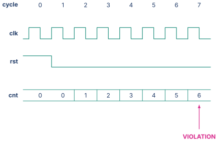
<Figure src="/figures/hardware-interview-prep/iv-19-Verification-Methodology-fig04.svg" alt="The counterexample is the shortest run that reaches the bad state, so every cycle it shows is part of the explanation and nothing in it is incidental traffic." caption="The counterexample is the shortest run that reaches the bad state, so every cycle it shows is part of the explanation and nothing in it is incidental traffic." id="fig:19-Verification-Methodology-4" />
That trace is **minimal**, because the tool finds the shortest path to the violation, so there is no irrelevant activity to wade through. Compare a simulation failure at cycle 4,200,000 whose cause was 900 cycles earlier under a pile of unrelated traffic. It is also **complete as a diagnosis**, because if no counterexample exists then none exists.
So a formal run has three outcomes and you must name all three. **Proven.** **Falsified**, with a counterexample. **Inconclusive**, meaning the tool ran out of time or memory and told you nothing at all. The third is the honest failure and the reason formal is not free.
### 5.4 Bounded versus unbounded, and proof depth
On a real design the fixed point often does not converge within budget, so tools also offer **bounded model checking**, asking the weaker question "is there a violation within the first $N$ cycles after reset." A bounded run that finds nothing returns "proven to depth $N$," and that number is the **proof depth**. It says no counterexample of length $N$ or shorter exists, which is not a full proof.
Whether that is worth anything requires thinking rather than quoting. Take a **16-entry FIFO** and the property "the write pointer never passes the read pointer." Constructing an overflow needs at least 17 writes with no reads, so at least 17 cycles. A bounded proof to **depth 10 proves literally nothing about overflow**, because the shortest possible counterexample is longer than the horizon searched. A proof to depth 40 covers fill, overflow attempt, drain, and underflow attempt with room, and that is real evidence.
The rule is to work out the **longest interesting sequence** in the block and require the depth to exceed it comfortably. For a FIFO that is its depth plus margin. For an 8-way round-robin arbiter it is at least 8 to complete a rotation and more like 20 under contention. For a cache controller it is the longest transaction, miss to fill to response, plus margin.
Two techniques extend the reach. **Abstraction** replaces a wide structure with a narrow one that preserves the property, for example shrinking a 512-entry buffer to 4 when the property does not depend on the count, which is often sound and always needs an argument. **Helper assertions**, sometimes called lemmas, are intermediate properties proven first and then assumed while proving the hard one, which is how a human writes a proof.
Whatever you get, **quote the depth when reporting**. "Proven" and "proven bounded to depth 12" are very different statements, and saying the first when the second is true is misreporting.
### 5.5 Over-constraining, the trap that eats projects
Formal must be told which inputs are legal, or it drives combinations the real system never produces and reports failures that cannot happen. So you write **assumptions**.
```systemverilog
// Fine. The environment never sends a request while reset is asserted.
no_req_in_rst: assume property (@(posedge clk) rst |-> !req);
// Catastrophic. "Fixing" a failure by assuming it away.
never_full_req: assume property (@(posedge clk) req |-> !full);
```text
You wrote the second because the tool kept producing counterexamples where a request arrived at a full FIFO and the design mishandled it. The assumption makes the failures stop. It also tells the tool **never to explore the case you were verifying**. Every subsequent proof on this block is silent about requests meeting a full FIFO, which is precisely where the bug was. The proof is green and worthless.
That is **over-constraining**, and its defining property is that it is **invisible in the results**. Under-constraining floods you with false failures, which is loud, annoying, and self-correcting. Over-constraining reports success, which is quiet and looks like progress.
Four checks, and knowing them is how you show real formal experience rather than tool familiarity. **Cover the assumption's antecedent**, meaning that for each meaningful assumption you write a `cover property` asking whether the interesting case is still reachable, so having assumed `req |-> !full` you check `cover property (full)`. **Run the vacuity check**, since an assertion `a |-> b` passes trivially whenever `a` is never true, and every tool has this check. **Prove assumptions on the driving block**, which is the strongest discipline and the one to name in an interview, meaning that if block B **assumes** `req` never asserts while `full`, then block A driving that signal must **assert** the same property, written once and included by both testbenches with `assume` in one direction and `assert` in the other, so the contract is verified from both ends and a later change to A fails A's own run instead of quietly falsifying B's proof. And **review the assumption list as a document**, because at the end of a formal effort that file is a specification of everything you believe about the environment, assumptions accumulate and nobody removes them, and the review is where you find the one somebody added in week 3 to unblock a run.
### 5.6 Where formal wins and where it dies
The rule is that **formal is strong where the state is small and the behavior is intricate, and weak where the state is large and the behavior is simple**. Control is the first. Datapaths are the second.
It wins on **arbiters**, where state is small, fairness and priority properties are subtle, request patterns are astronomically numerous, and "any requester holding its request eventually gets a grant" is a liveness property random simulation is genuinely bad at, per [Arbiters FIFOs and CAMs](/learn/hardware-interview-prep/arbiters-fifos-and-cams). It wins on **FIFO and queue control**, where the data is irrelevant to the properties so the storage abstracts away and the state collapses to pointers. It wins on **protocol interfaces**, proving handshake, ordering, and no-deadlock rules on an AXI or CHI port, per [Interconnect and AMBA](/learn/hardware-interview-prep/interconnect-and-amba). And it wins on **power management state machines**, where there are maybe 12 states, a dozen input conditions, catastrophic consequences if wrong, and enormous numbers of input orderings.
It dies on **wide datapaths**, where a 64-bit multiplier's reachable state is effectively all of it and functional correctness is a research-grade effort rather than a Tuesday. It dies on **large blocks**, since a whole core is thousands of times past any model checker's capacity. It dies on **properties needing long sequences**, where a 10,000-cycle violation is beyond bounded reach and unbounded will not converge. And it says nothing about **performance**, since it proves "a grant eventually happens" and not "throughput is 0.9 IPC," which is [Performance Modeling](/learn/hardware-interview-prep/performance-modeling) territory.
---
## Part 6, formal applications, the packaged uses
Tools also ship **applications**, formal engines wrapped around a pre-written property set for a common problem. They need little or no property writing, which makes them the easiest formal to adopt and the ones you may have used without calling it formal.
**Connectivity checking.** At SoC level there are tens of thousands of top-level connections, many of them one-bit control and status signals routed through several hierarchy levels. The spreadsheet says `soc_gpio[7]` connects to `block_c.io_out[3]` when `mux_sel == 2`. Nobody reviews that by eye and simulation only checks what a test happens to toggle. The application turns each row into a property and proves it with no stimulus, catching the integration bug class otherwise found in the lab. Directly relevant to the ASIC integration role.
**Register checking.** From an IP-XACT or RDL register map the application generates and proves that reset values are correct, that a read-only field never changes on a write, that a write-one-to-clear field clears on 1 and holds on 0, and that reserved bits read as zero. It replaces thousands of directed register tests and is more complete than they were.
**CDC and RDC.** Clock domain crossing checking from [Clocking Reset and Domain Crossing](/learn/hardware-interview-prep/clocking-reset-and-domain-crossing) is structural first, finding every crossing and confirming a recognized synchronizer is present, and formal second, proving the harder things such as "the data bus is stable while the crossing pulse is in flight" and "multi-bit control crossing together is gray-coded so only one bit changes at a time." Reset domain crossing is the same idea for resets, proving a flop reset by one reset does not feed a flop held out of reset by another during the window when they disagree.
**Deadlock and liveness.** **Safety** properties say nothing bad ever happens, which is everything above. **Liveness** properties say something good eventually happens, and they are a different animal, because a counterexample is not a finite trace but an infinite loop where the good thing never occurs.
```systemverilog
// safety
no_double_grant: assert property (@(posedge clk) $onehot0({gnt0, gnt1, gnt2}));
// liveness
req_gets_served: assert property (@(posedge clk) req0 |-> s_eventually gnt0);
```text
Deadlock checking asks whether the design can reach a state with no forward progress possible ever again. It matters most with multiple interacting queues and credit-based flow control, where deadlock arises from a **cycle of dependencies** rather than from any single block being wrong. Each block is individually correct, and A waits on B while B waits on C while C waits on A. Block-level testing never finds that, and random SoC simulation finds it only by constructing the exact circular condition by luck.
**Coherence protocols, the flagship.** If asked where you would apply formal on a cache project, this is the answer. A protocol from [Cache Coherence Protocols](/learn/hardware-interview-prep/cache-coherence-protocols) is defined by a stable MESI or MOESI state machine that looks small, and the real implementation is not, because every stable transition passes through **transient states** while a request is outstanding, and the transients dwarf the stable ones.
The bugs live in the interleavings. Core 0 issues a read-for-ownership for line X. While that is in flight core 1 requests X, and the directory sends core 0 an invalidate for a line core 0 does not yet own but has requested. Now add a writeback racing that invalidate in the opposite direction on a different channel with different latency.
Quantify why simulation is bad at it. Hitting a specific three-way race needs three events in a specific relative order within a few cycles. If each has a plausible timing window of 20 cycles, a specific ordering is around $1/20^2 = 1/400$ per opportunity, and the opportunity requires three cores targeting the same line at the same time. Multiply out and you are in the one-in-millions range, for a case that will absolutely happen in the field, because a shipped fleet executes $10^{15}$ cycles a day.
Formal handles it directly. Model 2 or 3 caches and 1 or 2 addresses, which suffices because coherence properties are per-line and symmetric, then prove the invariants. Two caches never hold the same line Modified at once. A line in Shared is never stale with respect to memory. Every request eventually receives a response. That state space is small enough to prove exhaustively, and the proof covers every interleaving including the ones nobody imagined. This is why coherence verification at every serious CPU company is formal-first.
---
## Part 7, equivalence checking
### 7.1 What it proves, and what it does not
**Logic equivalence checking**, universally LEC, takes two representations of a design and proves they compute the same function, typically your RTL against the netlist synthesis produced. It identifies **state points**, meaning flops and latches, in both designs and **maps** them to each other by name. That partitions each design into cones of combinational logic between state points, and for each corresponding pair it proves the Boolean functions identical. That is a pure combinational problem and therefore tractable at enormous scale, so a full core LEC run finishes in hours where formal property checking on the same core would never finish at all.
Now the thing that gets asked. **Equivalence checking proves nothing about whether your design is correct.** It proves the netlist matches the RTL. If the RTL has a bug, LEC will cheerfully prove the netlist reproduces that bug exactly, report full equivalence, and be right to.
So what is it protecting you from. **The tools.** Synthesis performs Boolean restructuring, resource sharing, constant propagation, retiming, clock gating insertion, scan stitching, buffer insertion, cell resizing, and hand-edited ECOs. Any of those could be implemented with a bug, or be **correctly** implemented but driven by a bad constraint, and the result is a netlist that does not do what your RTL did. Without LEC that difference is invisible until silicon comes back failing. You verified the RTL for nine months, and what tapes out is the netlist.
One sentence. **Simulation and formal verify the design. Equivalence checking verifies the flow that turned the design into a netlist.**
### 7.2 Where it sits in the flow
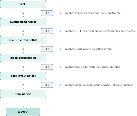
<Figure src="/figures/hardware-interview-prep/iv-19-Verification-Methodology-fig05.svg" alt="Every transformation on the way to tapeout is checked against the representation before it, so what LEC guards is the flow rather than the design." caption="Every transformation on the way to tapeout is checked against the representation before it, so what LEC guards is the flow rather than the design." id="fig:19-Verification-Methodology-5" />
The ECO run at the bottom saves the most careers. A last-minute engineering change order is often hand-edited into the netlist under time pressure at 2 a.m., and LEC against the corrected RTL is the only thing between that edit and the mask set.
LEC also finds real design problems rather than tool problems. When the RTL contains constructs simulation and synthesis interpret differently, LEC reports a mismatch, because the golden model it builds follows synthesis semantics. Incomplete sensitivity lists, a `casex` whose don't-cares synthesis treats as free choice, an inferred latch, and X-optimism in a `case` all surface this way, which is the [RTL Design and SystemVerilog](/learn/hardware-interview-prep/rtl-design-and-systemverilog) failure list arriving through a different door.
**Sequential equivalence checking** relaxes the state-point mapping that standard LEC needs and that breaks as soon as a transformation **moves** state. Retiming moves flops across logic, encoding changes rewrite an FSM from binary to one-hot, and pipeline insertion adds flops with no counterpart. Sequential LEC proves the two designs produce the same output sequences, usually allowing a fixed latency offset. It is much harder, closer to model checking than to combinational proof, and it stays a block-level activity.
---
## Part 8, running faster than a simulator
### 8.1 Simulation speed, quantified
An event-driven simulator on a full SoC runs at roughly **1 to 10 kilohertz** of simulated clock, a few thousand simulated cycles per wall-clock second. That number surprises people, so put it to work. Booting an operating system on a phone SoC is on the order of $10^{10}$ cycles.
| Platform | Speed | Time to boot |
|---|---|---|
| RTL simulation | 1 kHz | $10^7$ s = **116 days** |
| Fast simulation, small model | 10 kHz | 11.6 days |
| Emulation | 1 MHz | $10^4$ s = **2.8 hours** |
| FPGA prototype | 50 MHz | 200 s = **3.3 minutes** |
| Real silicon | 3 GHz | 3.3 s |
The software team must boot the OS, bring up the graphics stack, and profile real applications **before** silicon arrives, or the first year after tapeout goes to finding software problems that could have been found earlier. At 116 days per boot that is impossible. At 3 minutes it is routine.
### 8.2 Emulation and FPGA prototyping
An **emulator** is a large special-purpose machine, a rack of custom FPGAs or processor arrays, that compiles your netlist onto its fabric and runs at 1 to 5 MHz. What the money buys is **visibility**. It dumps full waveforms of any signal, has deep trace buffers, supports assertions and coverage, and can stop and inspect state. Transaction-level co-emulation lets the DUT run on the emulator while the UVM testbench runs on a workstation. It is a scheduled and contended resource, since a large emulator is a multi-million-dollar capital purchase with a data-center power budget and compile times in hours.
An **FPGA prototype** maps the design onto commercial FPGAs on a board at tens of megahertz, ten to fifty times faster than emulation at a tiny fraction of the cost, so software teams can each have one. The costs are equally concrete. **Debug visibility is poor**, since you see only the signals you decided in advance to route to a debug core, and changing that decision means a multi-hour rebuild. **Partitioning is hard**, because an SoC does not fit in one FPGA, so it is cut across several and the cut signals are time-multiplexed over limited board traces at a cost in performance and effort. **Memories and clocking need rework**, since ASIC SRAM macros and PLLs have no direct FPGA equivalent and must become block RAM and clock managers, which is a source of prototype-only bugs. And it models no timing, so nothing is learned about the real chip's frequency.
| | Emulation | FPGA prototype |
|---|---|---|
| Speed | 1 to 5 MHz | 10 to 100 MHz |
| Cost | millions | tens of thousands |
| Debug visibility | full, like a simulator | limited to pre-selected signals |
| Setup effort | moderate, largely automated | high, partitioning and memory mapping |
| Best for | hardware debug, coverage, early software | software development at volume |
### 8.3 Gate-level simulation
**Gate-level simulation**, GLS, runs the post-synthesis or post-layout netlist in an ordinary simulator with cell delays back-annotated from an SDF file. It is 10 to 100 times slower than RTL simulation and debugging it means reading waveforms full of machine-generated cell names. Everyone dislikes it and everyone runs it, because it catches things nothing else does.
**X-propagation problems.** RTL simulation is **X-optimistic**, often producing a defined value where real hardware produces an unknown. The classic case is a `case` on a selector that is X at time zero, where RTL simulation takes the default branch and produces something clean while the gates produce X that then spreads.
**Reset and initialization.** RTL testbenches routinely initialize state that hardware does not. In GLS every non-reset flop starts as X, so any logic quietly depending on a defined power-up value fails immediately. This is how you find the flop somebody left out of the reset tree.
**DFT logic behavior.** Scan chains, test mode muxes, compression logic, and the reset behavior of test structures do not exist in RTL. GLS is where scan shift and capture actually run, which connects to [DFT and Silicon Debug](/learn/hardware-interview-prep/dft-and-silicon-debug).
**Wrong timing exceptions.** With SDF back-annotated, a path declared a false path or a multi-cycle path in the SDC shows its real behavior. If the exception was wrong, per [STA Synthesis and Physical Design](/learn/hardware-interview-prep/sta-synthesis-and-physical-design), GLS can catch it where STA cannot, because STA obeyed the exception you gave it.
You cannot afford the whole regression in GLS. The answer to "how much" is a chosen subset, typically reset and boot, one test per major mode, the scan and DFT patterns, and the power state transitions.
---
## Part 9, what a design engineer owes verification
This is the framing an RTL interviewer is fishing for, and the wrong answer is "I write the RTL and they test it."
**Write assertions as you write the RTL, not afterward.** While writing the FIFO pointer logic you know at that moment that the write pointer must never pass the read pointer, and that knowledge is at its sharpest right then. Six weeks later you will not remember which invariants you relied on.
**Write down the corner cases you consciously handled and the ones you consciously did not.** If you decided a request during reset is illegal rather than handling it, that is a fact about the interface contract, and it belongs in the specification and eventually in an assertion on the driving block.
**Build the coverage model jointly.** You know which configuration bits interact and which are independent. The verification engineer does not, and left alone will cross everything with everything and produce a 4,000-bin report nobody can close.
**Review the verification plan yourself.** Reading someone's coverage plan for your block takes an hour and is the highest-value hour in the project, because you find the feature they did not know existed.
**Own the debug of failures in your block.** Handing one back with "the testbench is wrong" without looking is wrong about half the time.
**Identify formal-friendly pieces early and structure the RTL so formal can reach them.** A control FSM tangled into the same module as a wide datapath is much harder to prove than the same FSM in its own module behind a clean interface. Deciding that at design time is free. Retrofitting it is a rewrite.
**Do not fix a failure by weakening the property.** Establish which one is wrong first. This is the design-side version of the over-constraining trap in 5.5.
---
## Part 11, check yourself
Answer out loud, in full sentences, as an interviewer would hear them. If you cannot, reread the section named.
1. Quantify why a 64-bit adder cannot be exhaustively simulated, then explain what changes when you add 100 flops. (1.1, 1.2)
2. A colleague says formal is impossible because a block has $2^{100}$ states. What is the flaw, and where does the flaw stop applying? (1.3)
3. State precisely what a passing regression proves and what a passing formal proof proves. Why is that a difference of kind rather than degree? (1.4)
4. What is the exact ceiling of directed testing, and why does writing more directed tests not remove it? (2.2)
5. Your regression must hit a scenario with probability 1 in 5,000 per transaction. How many transactions for 95 percent confidence, and what do you do if the number comes out at a billion? (2.3)
6. Why must a reference model be written from the specification rather than the RTL? Describe a specific bug that becomes invisible otherwise. (2.4)
7. Name the UVM components and say which of the four testbench jobs each performs. Why must the monitor never consult the driver? (3.2, 3.3)
8. Give two situations where you would deliberately not use UVM, and justify each. (3.4)
9. Show a snippet with 100 percent line and branch coverage that is obviously untested, and say what code coverage fundamentally cannot see. (4.1)
10. Two coverpoints are at 100 percent and their cross is at 37.5 percent. Explain how, and what it means. (4.3)
11. Walk through the fixed-point reachability computation on a small counter. What does reaching a fixed point let you claim? (5.2)
12. You report "proven to depth 12" on a 16-entry FIFO's overflow property. Why is that worthless, and what depth would you need? (5.4)
13. Describe over-constraining, say why it is more dangerous than under-constraining, and give the four ways to check for it. (5.5)
14. Where does formal beat simulation and where does it fail? Give a concrete block for each. (5.6)
15. Why is cache coherence the flagship formal application, and can you quantify why simulation is bad at it? (6)
16. Equivalence checking passes on a netlist built from buggy RTL. Is the tool broken? What is LEC actually protecting you from? (7.1)
17. Booting an OS takes $10^{10}$ cycles. Work out the time on RTL simulation, emulation, and an FPGA prototype, and say which platform serves which purpose. (8.1, 8.2)
18. Name four things gate-level simulation catches that RTL simulation cannot, and say why you cannot run the whole regression in GLS. (8.3)
19. As the RTL owner of a block, what do you owe verification, and why is writing assertions later worse than writing them now? (9)
---
## Part 12, related notes
- [RTL Design and SystemVerilog](/learn/hardware-interview-prep/rtl-design-and-systemverilog) for assertion syntax, X-optimism, and the simulation-synthesis mismatch list that LEC and GLS surface
- [Clocking Reset and Domain Crossing](/learn/hardware-interview-prep/clocking-reset-and-domain-crossing) for CDC and RDC, the formal applications you have most likely already used without calling them formal
- [Cache Coherence Protocols](/learn/hardware-interview-prep/cache-coherence-protocols) for the transient states that make coherence the flagship formal target
- [Arbiters FIFOs and CAMs](/learn/hardware-interview-prep/arbiters-fifos-and-cams) for the arbiter fairness and liveness properties formal proves and simulation cannot
- [STA Synthesis and Physical Design](/learn/hardware-interview-prep/sta-synthesis-and-physical-design) for where equivalence checking sits in the implementation flow, and for the timing exceptions GLS can catch when they are wrong
- [DFT and Silicon Debug](/learn/hardware-interview-prep/dft-and-silicon-debug) for scan logic, which is only ever exercised in gate-level simulation, and for the post-silicon end of the debug story
- [Performance Modeling](/learn/hardware-interview-prep/performance-modeling) for the questions no technique in this note answers
- [Lab --- Verification and Cycle-Accurate Simulation](/learn/computer-architecture/lab-verification) for the vault's hands-on Verilator and riscv-formal material

Book mode