The Power Analysis Flow, from Activity Capture to Silicon Correlation
September 8, 202685 min readadvanced
Before any tool, do it manually. Take an 8-bit register. It holds a value, it gets clocked, sometimes the value changes. Here are twenty consecutive cycles of what it held, written in binary.
01.Part 1, what a power number actually is
1.1 Twenty cycles of one register, counted by hand
Before any tool, do it manually. Take an 8-bit register. It holds a value, it gets clocked, sometimes the value changes. Here are twenty consecutive cycles of what it held, written in binary.
| Cycle | Value | Bits that flipped since last cycle |
|---|---|---|
| 0 | 0000_0000 | n/a |
| 1 | 0000_0001 | 1 |
| 2 | 0000_0011 | 1 |
| 3 | 0000_0011 | 0 |
| 4 | 0000_0111 | 1 |
| 5 | 0000_0111 | 0 |
| 6 | 0000_0111 | 0 |
| 7 | 1111_1000 | 8 |
| 8 | 1111_1000 | 0 |
| 9 | 1111_1001 | 1 |
| 10 through 19 | held at 1111_1001 | 0 |
Add the last column. , so twelve bit-flips in twenty cycles, across eight bits, which is 160 bit-cycles of opportunity. So the average number of transitions per bit per cycle is .
Now convert that into power. From Power Fundamentals and Clock Gating, one complete round trip dissipates , half of it on the way up and half on the way down. Be careful with the attribution, because it is a thing interviewers probe. Only the rising half is actually drawn from the supply, and the falling half is the energy already stored on the node draining to ground. Averaged over a round trip that is of dissipation per transition in either direction, and that per-toggle figure is what every power tool bills. Take fF for the flop output and the small logic it drives, and V. Then one transition costs
Twelve of them is 12 fJ. Twenty cycles at 2 GHz is 10 ns. So the average power of this register's data side over this window is
That is a complete, exact power analysis. There is no approximation anywhere in it. And it required exactly two things, a number for the capacitance of each node and a count of how many times each node changed. Every power tool in existence, at every level of abstraction, from a spreadsheet to a signoff flow costing a million dollars a seat, is doing precisely this multiplication and nothing else.
1.2 The two ingredients, and only one of them is hard
Write the general form of what we just did.
where is the number of transitions node made during a window of length . That is it. That is the whole of dynamic power analysis.
The two ingredients are not equally difficult, and understanding why is the single most useful framing in this entire subject.
The capacitance is a property of the design. Once a netlist exists and the wires have been routed and extracted, is knowable to within a few percent from the standard cell library's characterization data and the extracted parasitics. It does not depend on what software runs. It does not change between Tuesday and Wednesday. It is a hard, static, engineering fact, and the flow that produces it is the one described in STA Synthesis and Physical Design.
The transition count is a property of the workload. It is not a property of the design at all. The same 8-bit register above, fed a different data stream, produces a different and therefore a different power. You cannot look at a schematic and read off any more than you can look at a car and read off its fuel consumption. You have to say what it is doing.
Everything difficult, contested, expensive, and interesting in power methodology is about . The rest of this note is very largely about how you get , how wrong it can be, and what happens when it is wrong.
1.3 Leakage, which does not fit the equation at all
The equation above has a window in it and counts transitions. Leakage, from section 1.4 of Power Fundamentals and Clock Gating, has neither. It flows whenever the block has supply, whether anything switches or not.
That gives leakage a completely different analysis character. It does not need activity at all. What it needs instead is state, meaning which logic value each node is sitting at, because a NAND gate leaks a different amount with inputs 00 than with 11, and temperature, because leakage roughly doubles per 10 degrees Celsius, and process corner, because a fast silicon lot leaks far more than a slow one.
So a real power report has two columns that are computed by two entirely different mechanisms, and a candidate who says "power analysis" without distinguishing them is going to get caught on the first follow-up. Keep them separate in your head from here on.
1.4 Average, peak, and why a number without a window is meaningless
Here is a trace of a block's instantaneous power over one microsecond.
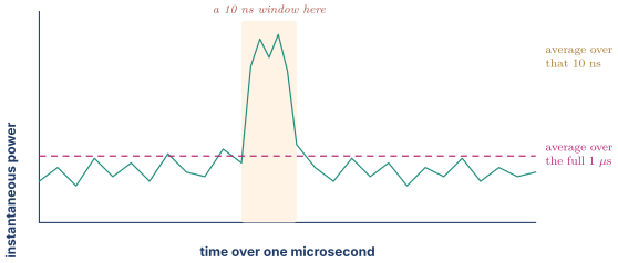
Three numbers come out of one trace. The full-window average is what sets battery life and what the heatsink or the phone chassis has to dissipate, because thermal mass smooths over microseconds. The narrow-window average across the burst is much higher and is what the power delivery network has to supply without the rail collapsing, which is the droop story in Part 4 of DVFS Droop and Thermal. And the energy for the whole task, which is average power times how long the task took, is what actually matters to a user, and it is the only one of the three that correctly rewards finishing sooner.
The practical consequence is a discipline of speech. A power number is not a fact until you have also said the workload, the window, the voltage, the frequency, the temperature, and the process corner. Say that unprompted in an interview and you have already separated yourself from most candidates, because it is the first thing a power lead has to teach every new hire and the tenth thing most candidates think of.
02.Part 2, vector-driven power estimation
2.1 A 4-bit counter, counted exactly
Take a free-running 4-bit binary counter and run it for 16 cycles, which is exactly one full wrap. Count the transitions on each output bit.
Bit 0 changes every single cycle, so 16 transitions. Bit 1 changes every second cycle, so 8. Bit 2 every fourth, so 4. Bit 3 every eighth, so 2. Total 30 transitions across 4 bits over 16 cycles.
| Bit | Transitions in 16 cycles | Transitions per cycle | , the rate |
|---|---|---|---|
| 0 | 16 | 1.000 | 0.500 |
| 1 | 8 | 0.500 | 0.250 |
| 2 | 4 | 0.250 | 0.125 |
| 3 | 2 | 0.125 | 0.0625 |
Take fF per bit including the logic each drives, V, GHz. Total transitions per cycle across the four bits is . So
That is an exact answer, and it is exact because we knew the stimulus completely.
2.2 Two conventions that differ by a factor of two, and one of them will bite you
Look hard at the third and fourth columns of that table. They differ by exactly two, always, for any signal that returns to where it started.
Power Fundamentals and Clock Gating uses meaning transitions per cycle, which is the convention that makes come out right, because one full round trip costs . EDA tools much more often speak of a toggle rate, meaning all transitions per cycle or sometimes transitions per nanosecond, and pair it with per transition, which gives the same answer by a different route.
Both are correct. Mixing them is a clean factor-of-two error in your power number, and it is invisible, because 2 times a plausible number is another plausible number. If you take one habit away from this section, take this one. Whenever anyone hands you an activity figure, ask which of the two it is before you use it. Interviewers who have run this flow will notice you asking.
2.3 What vector-driven power estimation is
Now the abstract definition, which after two worked examples is almost content-free. Vector-driven power estimation runs the design against specific stimulus, records what every node did, and multiplies the recorded transition counts by the capacitances. The "vectors" are the stimulus, whether they come from a directed test, a constrained-random regression from Part 2 of Verification Methodology, an emulated OS boot, or a trace replayed from a previous chip.
It splits into two flavours that differ in what they keep.
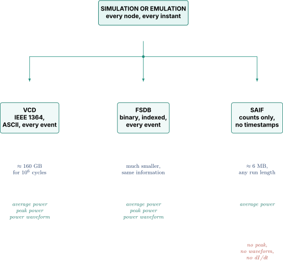
Averaged, or cumulative, vector-driven analysis. For each net, keep only the total transition count over the window and the fraction of time it spent at 1. That is one small record per net, and it is what a SAIF file holds. You get a single average power number, decomposable per instance, per block, per net, and split into internal, switching, and leakage components. You get no information about time.
Time-based vector-driven analysis. Keep every event with its timestamp. That is what a VCD or an FSDB holds. Now the tool can produce a power waveform, so you can ask what the power was during cycle 4,912,338, find the peak window, and hand to the power-integrity people for the droop analysis in Part 4 of DVFS Droop and Thermal. The cost is that the activity file is orders of magnitude larger and the analysis is far slower.
Synopsys documents both modes on PrimeTime PX and PrimePower, describing average power analysis driven by SAIF or user-specified activity, and peak power analysis requiring a VCD that captures the time of every event. Cadence's Joules is marketed specifically on time-based RTL power. Nothing about that split is vendor-specific, it falls straight out of what the activity file kept.
2.4 The error vector-driven analysis introduces, which is not what people expect
Ask an interviewer's favourite trick question of yourself. If vector-driven analysis is exact, where does its error come from?
It is not modelling error. Given the stimulus, the tool's answer is essentially the truth, subject only to how good the capacitance and cell models are. The error is representativeness. The answer is exactly right for the vectors you ran, and the vectors you ran are almost never the workload the chip will actually see.
Make it concrete with the counter. Suppose your directed test happens to hold the counter's enable low for 12 of the 16 cycles because it was written to check something else. Now bit 0 makes 4 transitions instead of 16, and your measured power is a quarter of the free-running figure. Nothing is wrong with the tool. The number is a true fact about a test that has nothing to do with how the counter behaves in the product.
Three further sources of error sit underneath that main one and are worth naming because each has a different fix.
Unknowns. A net that is X in simulation has no defined transition count. Tools variously ignore such nets, assume a default, or propagate the X, and a design with a lot of X at the start of a run can quietly lose a chunk of its activity. Fixing it means fixing the reset and initialization behaviour, which is the gate-level simulation story in section 8.3 of Verification Methodology.
Glitches. From Digital Logic and Timing, which is where note 17 sends you for this, a combinational node can make several transitions on its way to the right answer, and each one costs energy. Whether your activity capture sees those depends entirely on whether the simulation had real delays in it. A zero-delay RTL simulation cannot see a glitch, because in a zero-delay model the wrong intermediate value never exists. So glitch power is a term that RTL-derived activity structurally under-counts, and it under-counts it in the dangerous direction.
Window choice. If you average over a window that includes a long idle stretch, you get a small number that is true and useless. Choosing the window is a modelling decision that belongs to the engineer, not the tool.
03.Part 3, vectorless power estimation
3.1 Two gates, and the assumption that fails
Vectorless estimation runs no stimulus at all. Instead it assigns each primary input a signal probability, meaning the fraction of time it is at logic 1, and a transition density, meaning how often it changes, and then propagates those statistically through the logic. The idea is due in its modern form to Najm's transition-density work, and every commercial vectorless engine is a descendant of it.
Watch it work on two gates, and then watch it fail on three.
Take an AND gate with inputs and . Say each is at 1 half the time, so , and say they are independent. Then
That is right, and you can check it by hand against the four rows of the truth table. Now build this instead.
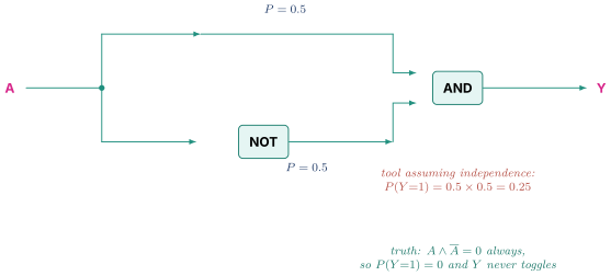
The final AND's two inputs both descend from . They are not independent, they are perfectly anti-correlated, and the output is a constant zero that never toggles and burns no dynamic power at all. A propagation engine that multiplies probabilities reports 25 percent occupancy and a healthy toggle rate, on a wire that is nailed to ground.
This structure has a name, reconvergent fanout, and it is not a contrived corner case. It is everywhere, in every mux select tree, every one-hot decoder, every enable network, every carry chain. The academic literature on limited-depth reconvergence analysis exists precisely because ignoring it is unacceptable and handling it exactly is intractable. Commercial engines handle correlation to a bounded depth and give up beyond it, on the reasonable argument that signals reconverging after many levels of logic are close enough to independent that the residual error is small.
3.2 What vectorless estimation actually computes
With the failure mode in hand, the definition lands properly. Vectorless power estimation assigns statistical activity to a chosen set of nodes, usually the primary inputs and the register outputs, and propagates it through the logic using a probabilistic model, producing an estimate with no simulation anywhere in the flow.
It computes an expected power under an assumed statistical model of the inputs. It is not an approximation of the power under your workload. It is the exact power of a hypothetical, statistically-described workload that may or may not resemble yours, computed under an independence assumption that is definitely violated somewhere in your netlist.
Three distinct errors stack up in it, and being able to separate them is the discriminating answer.
Input assumption error. You told it 0.2 toggles per cycle. The real workload does something else. This is usually by far the largest term and section 3.3 quantifies it.
Correlation error. The reconvergence problem above, plus temporal correlation, meaning the fact that real data is not memoryless. Bus addresses walk upward in small steps, video pixels resemble their neighbours, and instruction opcodes are drawn from a skewed distribution. The independence-in-time assumption fails as hard as the independence-in-space one.
Glitch error. Probabilistic propagation with a zero-delay model has the same blindness as zero-delay simulation, and tools that model glitching statistically do so with a further layer of assumption.
3.3 A toggle-rate assumption producing a confidently wrong answer
This is the worked example to have ready, because "give me an example where a default toggle rate misled you" is a question a power lead will actually ask.
Set up a block. Two hundred thousand switching data nodes, effective capacitance 3 fF each, so pF. Supply 0.8 V, clock 2 GHz. Then
The flow's global default for un-annotated data nets is a toggle rate of 0.2 per cycle, meaning in the note-17 convention. So the tool reports
for any block of this size and technology, regardless of what it does. That is the whole problem in one sentence.
Now take two real blocks of exactly that size.
Block V, a video line buffer. Its data is pixel samples from adjacent scanlines, which are strongly correlated, so the high-order bits barely move while the low-order bits are noisy. Measure it and three quarters of the nodes sit at and one quarter at . The weighted activity is
The default over-estimated it by 29 percent. Annoying, wasteful, but safe.
Block C, a cipher datapath. Its intermediate values are designed to look like uniform random bits, which is the entire point of the primitive. Every node sits near .
The default under-estimated it by a factor of 2.5. You budgeted 77 mW and the block draws 192.
Now the part that makes this a good story rather than a good arithmetic exercise. Roll it up. Suppose the chip has seven blocks like V and one like C.
| Default assumption | Reality | |
|---|---|---|
| Seven video-class blocks | mW | mW |
| One cipher block | mW | mW |
| Chip total | 614.4 mW | 608.5 mW |
The chip-level number is wrong by 0.95 percent. It looks like a triumph. The power lead signs it off, the thermal model is built on it, the battery-life projection is built on it, and every one of those is fine.
And the cipher block is at two and a half times its budget. That block's local power grid was sized for 77 mW, so its IR drop is far outside what was assumed. It is a thermal hotspot the floorplan did not anticipate. Its switch-in transient is 2.5 times the assumed , which is the droop mechanism of Part 4 of DVFS Droop and Thermal, and the droop it creates lands on every other block sharing the rail.
Say the moral out loud, because it is the reusable part. Errors from a global toggle-rate default are not random noise that averages out. They are systematic, they are correlated with what the block does, and a chip total that comes out right can be right for two large wrong reasons that happened to cancel. A power methodology that only checks the total is not checking anything.
3.4 When vectorless is nonetheless the right tool
Having taken it apart, be fair to it, because a candidate who only knows the criticism is as unbalanced as one who only knows the marketing.
When no vectors exist yet. At early RTL, before the testbench is written, before anything boots, vectorless is the only thing available. A wrong number today that steers an architectural decision correctly beats a right number in nine months when the decision is frozen.
For relative comparison. If you are choosing between a 4-read-port register file and two banked 2-port ones, both estimates carry the same systematic bias, and the bias largely cancels in the ratio. Vectorless is far more trustworthy on "A is 40 percent less than B" than on "A is 82 mW."
For leakage. Leakage barely depends on activity. A vectorless leakage number at a stated corner and temperature is a genuinely good number.
For finding structure rather than magnitude. The most valuable RTL-stage power reports are not power numbers at all, they are lists. Registers with no clock gating enable. Memories being read on cycles where the result is discarded. Datapaths toggling behind a disabled valid. Those findings do not depend on the activity assumption being right, and they are exactly what the SpyGlass Power and PowerArtist reduction reports in Part 8 are built to produce.
And, most importantly, in hybrid form. The real flow is almost never purely vectorless. You annotate the activity you know, typically at block boundaries, on clocks, on memory interfaces, and on any signal a designer can state a fact about, and let the engine propagate statistically only into the interior. That collapses the input-assumption error, which was the dominant term, and leaves only the correlation error, which is the smaller one. If you are asked "vector-driven or vectorless," the strong answer names the hybrid and explains why the hybrid attacks the larger of the two error terms.
04.Part 4, activity capture, the formats and where they come from
4.1 VCD, and the size problem that motivates everything else
VCD, Value Change Dump, is the plain-text activity format defined as part of the Verilog language standard, IEEE 1364. It is ASCII, it is universally supported by every simulator ever shipped, and its content is exactly what its name says. A header declaring the signals and their short codes, then a stream of timestamps, and after each timestamp the new value of every signal that changed at that instant.
Its virtue is that it is complete and portable. Its problem is arithmetic. Size the file for a real run.
Take 100,000 dumped nets at an average of 0.2 transitions per cycle, so 20,000 value-change records per cycle. Each record is a value plus an identifier plus a separator, call it 8 bytes with short codes. Run for cycles, which at 2 GHz is half a millisecond of chip time and is a short run.
Half a millisecond. One hundred and sixty gigabytes. Now consider that a realistic software workload is to cycles and the number goes to petabytes. Writing it would dominate the simulation runtime even if you had the disk.
That single calculation is why the other two formats exist, and it is worth being able to produce on a whiteboard.
4.2 SAIF, and the trade it makes
SAIF, the Switching Activity Interchange Format, solves the size problem by throwing away time. It is still ASCII, it is hierarchical and mirrors the design hierarchy, and for each net it records a small fixed set of numbers rather than a stream of events. The standard fields are the toggle count and the durations spent in each logic state, conventionally written TC for the number of transitions, T0 and T1 for time spent at zero and one, and TX for time spent unknown. Set-and-reset statistics for sequential elements appear as well.
SAIF originated as a Synopsys format and is now described in an annex of the IEEE 1801 low-power standard, the same standard that carries UPF. I would not quote the annex letter or the exact edition in a room without checking it, and neither should you, but "it is documented in an annex of 1801" is safe and shows you know it was standardized rather than staying proprietary.
Now the size, for the same run as above.
Six megabytes against a hundred and sixty gigabytes. And here is the property that matters most and that people miss. The SAIF file's size does not depend on how long you simulated. Run for ten times as long and the counters get bigger, the file does not. A SAIF from a billion-cycle emulation run is the same six megabytes as one from a thousand-cycle unit test.
What you gave up is everything time-dependent. No peak power. No power waveform. No . No answer to "when in the run did that happen." SAIF answers "how much on average," and it answers nothing else.
Forward and backward SAIF is the second thing to know, and it is the detail that signals flow experience rather than reading. The problem it solves is names. Your activity was captured against RTL signal names. Your power analysis runs on a synthesized netlist where those names have been optimized, merged, renamed, and in many cases deleted. Annotating a gate-level netlist from an RTL SAIF is therefore a name-mapping problem.
The classical Synopsys solution is a two-pass handshake. The synthesis tool writes a forward SAIF, produced from the elaborated design, which tells the simulator which objects to monitor and in what naming scheme. The simulator monitors exactly those and writes a backward SAIF holding the measured TC, T0, T1, TX values. The synthesis or power tool reads the backward file and annotates. Along the way you have to preserve RTL hierarchy names through synthesis or the mapping fails silently and you get an analysis where a large fraction of nets fell back to defaults, which lands you straight back in section 3.3.
Here is the practical instinct to carry. After any annotation step, read the tool's annotation-coverage report before you read the power number. If 40 percent of nets were not annotated, your power number is 40 percent vectorless with default activity and you did not know it.
4.3 FSDB, and what buying a binary format gets you
FSDB, Fast Signal Database, is the binary waveform format originally from Novas, which passed to SpringSoft and then to Synopsys, and is the native database of the Verdi debug environment. It is proprietary, so precision about its internals is not available and you should not claim any.
What is publicly described and safe to say is the shape of the trade. It is compressed and indexed rather than a flat text stream, so it is substantially smaller than VCD for the same content, with vendor and community figures commonly quoted in the region of five to ten times, which will obviously vary with the design and the signal set. It supports random access, so a viewer can jump to cycle nine hundred million without reading the preceding nine hundred million. It supports incremental reading while the simulation is still running. And it carries more than pin values, including assertion results and transaction-level records, which is why it became the debug format rather than merely a power-input format.
For power purposes the important property is that FSDB keeps time, so it can drive time-based analysis and peak power the way VCD can, at a fraction of the storage. That is why a modern time-based power flow tends to be FSDB-driven rather than VCD-driven even though VCD is the standard.
4.4 Where the activity comes from, part one, simulation and its hard ceiling
Section 8.1 of Verification Methodology gives the number that governs everything here. An event-driven simulator on a full SoC runs at roughly 1 to 10 kilohertz of simulated clock.
Put a workload against it. A modern software workload worth profiling for power, a video decode of a few seconds, a camera capture pipeline, a benchmark run, a browser page load, is on the order of to cycles.
Eleven and a half days for the shortest interesting workload, and that is before you account for the slowdown of dumping activity, which is not small.
So the ceiling is not a matter of patience or budget. Simulation-derived activity is structurally incapable of representing a real workload. What it can represent is a directed scenario of a few thousand to a few hundred thousand cycles. That is genuinely useful for a block, and it is the right tool for "what does this FIFO burn while draining at full rate," but it can never answer "what does the chip burn playing a video."
Do not let that be read as dismissive. Almost all block-level power work, all of the clock-gating opportunity hunting, and all of the early per-instance reports run on simulation-derived activity, and they should. The ceiling is about full-chip workload power, not about power analysis in general.
4.5 Where the activity comes from, part two, emulation and why it changed the game
An emulator, per section 8.2 of Verification Methodology, runs the netlist on a rack of purpose-built hardware at roughly 1 to 5 megahertz. Redo the division.
Eleven days becomes seventeen minutes. That is a factor of a thousand, and factors of a thousand do not make an existing activity better, they create activities that did not exist. The one they created here is profiling the power of real software on pre-silicon hardware.
Every major emulation vendor now ships a power application on top of the emulator for exactly this. Cadence has Dynamic Power Analysis on the Palladium platforms, Synopsys has ZeBu Empower, and Siemens pairs the Veloce Power App with PowerPro for emulation-driven power. All three publish claims about billion-cycle capability and about accuracy in the mid-to-high nineties percent against their own signoff reference. Cadence's public number for Palladium DPA, for instance, is up to 97 percent. Treat those percentages as vendor claims measured under vendor-chosen conditions, name the products because these roles screen on the vocabulary, and do not repeat the percentages as if they were physics.
The interesting part is not the marketing, it is the shape of the flow, which is forced by section 4.1's file-size arithmetic. You cannot dump full-fidelity activity for a billion cycles, because that is the petabyte case. So the flow is two-phase, and being able to describe the two phases is the answer that shows you understand rather than recognize.
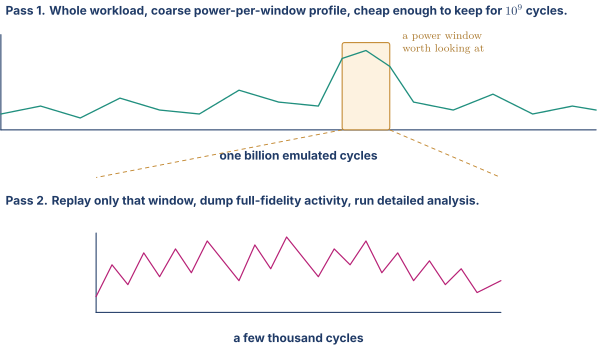
Pass one runs the entire workload with a lightweight, always-on activity accumulator, producing a coarse power-versus-time curve at, say, one point per few thousand cycles. That is cheap enough to keep for the whole run. Pass two takes the windows the curve flagged, replays just those, and dumps full activity for detailed per-instance analysis.
Then say what actually changed, because the two-phase flow is the mechanism and this is the consequence. Power stopped being a property you estimate and became a property you profile. Before emulation-driven activity, the question you could answer was "what does this test burn." After it, the question is "which two hundred microseconds of the camera pipeline burns the most, what is running then, and which block is responsible," which is the same shape of question a performance engineer has been able to ask for thirty years, per Performance Modeling. It also made power a software finding. A driver polling a register at a kilohertz, a firmware loop that never lets a domain reach the residency threshold from section 6.3 of Power Fundamentals and Clock Gating, a memory access pattern that defeats a power-saving mode, are all now visible before tape-out, and all of them are fixed in software at a thousandth of the cost of fixing them in silicon.
05.Part 5, the accuracy-versus-maturity curve
5.1 Four stages, and what each one can and cannot tell you
Power gets estimated at four broadly distinguishable points in the flow, and they differ in what physically exists at that point.
RTL power estimation. No netlist exists. The tool synthesizes a fast internal estimate of what the gates and wires would be, or uses calibrated models built from previous designs, and applies activity from RTL simulation or from vectorless propagation. Ansys builds PowerArtist's accuracy story around exactly this, with a calibration step it calls PACE that starts from a post-layout design and produces RTL power models that track it. Cadence positions Joules on the same premise, generating gate and wire estimates from the production implementation technology rather than from generic assumptions.
Gate-level, post-synthesis, without annotated activity. A netlist exists. Capacitance is real for cells and estimated for wires, since routing has not happened. Activity is vectorless or default. This stage is much more precise about the design and no better at all about the workload, which is worth sitting with, because it is where a lot of false confidence is manufactured.
Gate-level with annotated activity. The same netlist, now with activity back-annotated from a simulation of the netlist itself. If that simulation carried real cell delays, glitch power appears for the first time.
Post-layout signoff. Routing is done, parasitics are extracted, the clock tree is built and real, and the analysis runs with the actual capacitances at the actual operating conditions. This is the number the project commits to.
Error bands are where the literature and the vendors disagree, so hedge honestly rather than inventing. Two figures are safe because they are published and attributable. Cadence's launch material for the Joules RTL Power Solution claims gate-level accuracy within 15 percent of final power as signed off in Voltus, and Ansys claims out-of-the-box RTL clock power within 10 to 15 percent of signoff for 10 nm designs, using the PACE calibration flow and the RTL clock-tree synthesis engine inside it. Both are vendor claims under vendor-chosen conditions, and both are about correlating a tool to another tool from the same vendor rather than to measured silicon. Numbers for the harder target, correlation against a real part, circulate as rules of thumb in the region of a few percent at gate level and low tens of percent at RTL, but I would not quote a specific figure for those without a source in hand, and neither should you. My honest position, and the one to state in a room, is that the achievable band depends far more on how well your RTL model has been calibrated against your own previous silicon than on which vendor's logo is on the tool, and that anybody quoting a single universal percentage is quoting a marketing slide.
| Stage | What exists | What it tells you well | What it cannot tell you | Rough band, hedged |
|---|---|---|---|---|
| RTL estimation | RTL only | relative comparison of architectures, gating opportunities, where the power is by block | absolute compliance with a tight budget | order 15 percent, heavily calibration-dependent |
| Gate-level, no annotation | netlist | structural power distribution, leakage by cell type | anything workload-dependent | design-accurate, workload-blind |
| Gate-level, annotated | netlist plus delays | glitch power, realistic per-instance ranking | routing capacitance, real clock tree | better, still pre-route |
| Post-layout signoff | everything | the committed number, peak windows, per-rail totals | it arrives too late to change anything cheaply | tightest band available pre-silicon, but still bounded by workload representativeness rather than by the tool |
5.2 The real axis is not accuracy, it is which decision the number can support
Accuracy is the wrong thing to optimize and the wrong thing to talk about. Here is the framing that a power architect will recognize immediately.
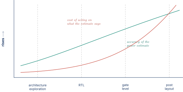
The two curves run the wrong way relative to each other, and that is the central tension of the whole discipline. The decisions with the largest power leverage, meaning how many execution ports, how wide the vector unit, how many cache ways, whether a unit gets its own power domain, are all made where the numbers are worst. By the time the numbers are trustworthy, changing any of those costs a schedule slip.
So the goal at the RTL stage is not accuracy. It is decision-preserving fidelity, meaning the estimate ranks the options in the same order the signoff tool eventually will. An RTL flow that is consistently 18 percent high but always ranks correctly is worth more than one that is 6 percent off on average and occasionally inverts two options.
And that is exactly why calibration, of the PACE flavour, is worth the effort it costs. Calibrating an RTL model against your own last chip's post-layout data removes the systematic component of the error, which is the part that inverts rankings, and leaves the random component, which mostly does not.
5.3 The clock tree, which is the largest term and the least knowable early
One specific consequence of section 5.2 deserves its own paragraph because it is the most quotable single fact in this note.
Section 2.1 of Power Fundamentals and Clock Gating establishes from first principles that the clock network is roughly a third of dynamic power in a typical block. Now notice when the clock network comes into existence. Clock tree synthesis happens in physical design, well after RTL and after logic synthesis. So the single largest term in the power budget is the one term that does not physically exist at the point where the budget is being set.
That is why RTL power tools invest specifically in clock tree modelling, estimating buffer counts, levels, and wire lengths before CTS runs, and why vendor accuracy claims are so often stated for clock power specifically. It is also why a badly estimated clock tree can wreck an otherwise good early projection all by itself, and why "what did you assume about the clock tree" is a fair and pointed question to ask of any RTL power number, including your own.
5.4 Two things a netlist alone still cannot give you
Wire capacitance. At advanced nodes interconnect is a large share of the switched capacitance and its value depends on the route, which depends on placement, congestion, and the metal stack. Post-synthesis estimates come from wire-load models or from virtual routing, and both are estimates. Extraction after routing is what turns them into measurements.
Glitch power. A zero-delay netlist simulation cannot produce a glitch, so the glitch term is missing from every stage until you run a delay-annotated simulation. Because glitch power only ever adds, this is a systematic under-estimate, and it is the classic reason a project's power number drifts upward as it matures rather than jittering around a fixed value. If someone shows you a project where every re-estimate came in higher than the last, unmodelled glitch is one of the first three things to suspect.
06.Part 6, per-block budgeting and rollup
6.1 A six-block chip, budgeted by hand
Budgeting is where power methodology stops being a tool question and becomes an organizational one, and interviewers for principal and architect roles care about it more than about any file format.
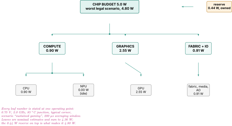
Start concrete. A chip has a sustained power target of 5.0 W at its thermal design point. Six blocks have been characterized at their individual peaks.
| Block | Peak power |
|---|---|
| CPU cluster | 2.4 W |
| GPU | 2.8 W |
| Neural accelerator | 1.6 W |
| Media, encode and decode | 0.7 W |
| Fabric and memory controller | 0.9 W |
| Always-on and miscellaneous | 0.1 W |
| Sum of peaks | 8.5 W |
The sum of the peaks is 8.5 W against a 5.0 W target, which is 70 percent over. A naive reading says the chip is impossible and three blocks have to be cut.
That reading is wrong, and seeing why is the whole of budgeting. A chip budget is not the sum of block maxima. It is the maximum over the legal concurrent scenarios. Blocks do not all peak at once, because software does not ask them to, and the ones that could be asked to are prevented from doing so by a runtime power manager.
Write the scenarios down.
| Scenario | CPU | GPU | NPU | Media | Fabric | AO | Total |
|---|---|---|---|---|---|---|---|
| Sustained gaming | 1.0 | 2.8 | 0.0 | 0.1 | 0.8 | 0.1 | 4.8 W |
| Camera capture with on-device inference | 0.8 | 0.5 | 1.6 | 0.7 | 0.7 | 0.1 | 4.4 W |
| CPU burst benchmark | 2.4 | 0.2 | 0.0 | 0.0 | 0.6 | 0.1 | 3.3 W |
| Video playback, screen on | 0.3 | 0.4 | 0.0 | 0.6 | 0.5 | 0.1 | 1.9 W |
| Everything at maximum simultaneously | 2.4 | 2.8 | 1.6 | 0.7 | 0.9 | 0.1 | 8.5 W |
The worst legal scenario is gaming at 4.8 W, which fits inside 5.0 W with 0.2 W, about 4 percent, of headroom. The chip is feasible.
The last row is the one that matters most for the reader of this note. Nothing in the silicon prevents all six blocks from running flat out at the same time. What prevents it is a runtime power manager that refuses to grant the concurrent request, by capping frequency, denying a power-up, throttling an accelerator, or delaying a wake. The last row is not a design bug, it is a requirement on a control block, and that control block is exactly the class of thing a power-management designer builds.
6.2 Margin, and why hidden margin is worse than no margin
Every number in that table is uncertain, so every number carries margin. The question is where the margin lives, and it has a right answer.
Suppose the true nominal gaming scenario is 4.36 W and each of the six block owners, sensibly, carries 10 percent inside their own reported figure. The reported total is W, which is the number in the table.
Now suppose instead the block owners report 4.36 W nominal and the integrator holds a single explicit 0.44 W reserve. The total is identical. Everything else about the two situations is different.
When the GPU comes in 0.6 W over, the second arrangement lets you spend a reserve that everyone can see and someone owns. The first arrangement leaves you with 0.44 W of margin distributed invisibly across six people's numbers, which you cannot spend because nobody knows it is there and no owner will admit to holding any.
Worse, margin compounds when it is hidden. If each block carries 10 percent and the integrator, not knowing that, adds another 10 percent at the top, the stack is , so 4.36 W is reported as 5.28 W. The chip is now over budget on paper by 0.28 W and the team will spend real months and real area optimizing a problem that does not exist. That failure mode is common, it is expensive, and it is entirely a communication failure rather than an engineering one.
The rule that follows is short. Margin should be explicit, singular, and owned. Blocks report their best estimate and, separately, their uncertainty. The integrator holds one visible reserve sized against the aggregate uncertainty. Whether that reserve is a plain sum of block uncertainties or something smaller is a judgment call about how independent the uncertainties are, and it is a place to be careful. A root-sum-square reduction is defensible for genuinely independent random errors, and completely indefensible for the systematic errors of section 3.3, because a shared wrong toggle-rate default biases every block the same direction at once. If you use RSS, say what makes the errors independent.
6.3 The rollup bug that catches everybody
Here is the single most common technical error in power rollup, and it has nothing to do with tools.
Block A reports 0.40 W. Block B reports 0.40 W. Someone adds them and writes 0.80 W. But A was characterized at 0.75 V and 85 degrees Celsius, and B at 0.90 V and 25 degrees.
Convert B to A's conditions. Dynamic power scales with , so
meaning B's dynamic component would be about 31 percent lower at A's voltage. Leakage runs the other way and much harder. Using the conservative factor of 1.7 per 10 degrees from section 1.4 of Power Fundamentals and Clock Gating, going from 25 to 85 degrees is six doublings-ish,
so B's leakage at A's temperature is roughly twenty-four times what was reported. If B was 0.35 W dynamic and 0.05 W leakage at its stated conditions, then at A's conditions it is about W. The honest total is not 0.80 W, it is about 1.84 W, more than double.
One honest correction to that arithmetic, and volunteering it is worth more than the arithmetic itself. The temperature term above is applied on its own, but B is also moving from 0.90 V down to 0.75 V, and leakage is strongly voltage-dependent too, through drain-induced barrier lowering rather than through the that governs dynamic power. Dropping the supply by that much typically cuts subthreshold leakage by something on the order of a factor of two, so the true multiplier is not 24 but appreciably less. Redo it with twelve rather than twenty-four and B lands at W, so the defensible total is somewhere near 1.2 W rather than 1.84 W. Note what did not change. The naive answer of 0.80 W is still badly wrong, and it is wrong in the unsafe direction. A real conversion uses the library's own leakage tables at the target voltage, temperature, and corner rather than a doubling rule applied to one variable at a time. The doubling rule is a whiteboard sanity check, not a normalization method, and saying so is what stops an interviewer concluding you learned this from a slide.
The lesson generalizes past the arithmetic. A power number carries a conditions vector, and adding two numbers taken at different conditions is not addition, it is nonsense. So the rollup discipline is that every contributing number is normalized to one stated operating point before anything is summed, and the operating point is written at the top of the sheet where nobody can miss it. Every mature power team enforces this with a template, and the reason the template exists is that this exact mistake has cost someone a tape-out.
6.4 What happens when a block overruns
The GPU comes back at 3.4 W instead of 2.8, three months before tape-out. Gaming goes to 5.4 W against a 5.0 W target. What now?
There is a ladder, and it runs cheapest first. Being able to recite it in order is a good architect-level answer, because it demonstrates that you know the expensive options exist and that you know they are last.
Step zero, and skip it at your peril. Determine whether the design got worse or the model got better. A 0.6 W jump between two estimates is very often a methodology change, a newly annotated glitch term, a corrected clock-tree assumption, a different activity source, a different corner. Rerun the old configuration alongside the new one and difference them. Optimizing a block against a number that moved for measurement reasons is pure waste, and it happens constantly.
Step one, recover activity. Per-instance reports sorted by power, exactly the procedure in section 4.1 of Power Fundamentals and Clock Gating. Ungated registers, un-isolated operands, memories read speculatively and discarded, datapaths toggling behind a dead valid. These are RTL edits with no architectural consequence and they are where the first tranche of savings usually is.
Step two, coarser gating and domain restructuring. Can a whole sub-unit be clock gated on an architectural idle condition? Does it deserve its own power domain? Both cost design effort and verification effort, and the domain option costs area and sequencing complexity per Part 7 of Power Fundamentals and Clock Gating.
Step three, microarchitecture. Fewer ports, narrower issue, smaller structures, a banked instead of a monolithic array, a different arithmetic algorithm per Arithmetic Hardware. Real performance is on the table now, and this is where the conversation stops being a power conversation and starts being a product one.
Step four, spend the reserve. This is why section 6.2 insisted the reserve be visible. It is a legitimate move and it is finite.
Step five, move the operating point. Cap the GPU's frequency and voltage. Very effective, because of the term, and it directly costs the performance the block existed to provide, per Part 1 of DVFS Droop and Thermal.
Step six, change the specification. Lower the sustained target, accept a shorter turbo window, revise the thermal design, change the product's claimed battery life. This is a business decision, and it is above your pay grade, but noticing that it is an option and escalating early rather than late is very much not.
07.Part 7, pre-silicon to silicon correlation
7.1 What you can actually measure on a real part
The first thing to get straight is that you do not measure a block. You measure a rail.
Instrumentation comes in a few flavours, all public knowledge. Off-chip, a sense resistor in series with a supply rail on the board or on a characterization fixture, with the voltage across it giving current. Regulator telemetry, where the power management IC reports its own output current, cheap and always available and typically the least accurate. And on-die sensors, which vary enormously between products and about which I would say nothing specific in an interview beyond that they exist.
Whatever the mechanism, the granularity is the rail. If the CPU cluster, its L2, and part of the fabric share a rail, the measurement gives you their sum and nothing finer. To decompose you have to change the experiment, by holding blocks in reset, running stimulus that exercises one block at a time, or comparing two workloads that differ in exactly one activity. That constraint is why power-aware floorplanning of rails is partly a debug decision, and noticing that out loud is a strong signal.
So the raw correlation event is unglamorous. Projection said 2.6 W on this rail under this workload. Silicon says 3.2 W. There is 0.6 W of discrepancy and it is currently one undifferentiated lump.
7.2 Splitting the lump, the frequency sweep
Here is the technique that turns one number into two, and it comes straight out of the physics in Part 1 with no tooling at all.
Total power on a rail is dynamic plus leakage.
Hold the voltage fixed, hold the temperature fixed, run the same workload, and vary only the frequency. Then and are both constants and the expression is a straight line in whose intercept is the leakage and whose slope is the effective switched capacitance times .
Measure two points. At 0.80 V, junction held at 50 degrees, running a fixed compute loop:
Now back-substitute at the 1 GHz point, keeping the units honest, because the slope is joules per cycle and only becomes watts once it is multiplied by a frequency.
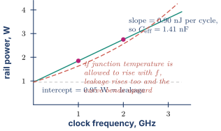
Now you have two numbers to compare against two projections instead of one against one, and the diagnosis forks cleanly.
If leakage matches and dynamic is high, it is an activity problem or a capacitance problem. Activity is far more likely, so look at the workload mismatch first, then glitch, then the clock tree.
If dynamic matches and leakage is high, it is not an activity problem at all. Suspect the process corner of the parts you were given, the actual junction temperature versus the assumed one, the multi-Vt mix that synthesis finally chose versus the one that was assumed, and whether the domains you believed were powered off actually were.
If both are high by similar ratios, suspect something global. The voltage the part is really running at rather than the nominal, given the guardbanding in Part 3 of DVFS Droop and Thermal. Or the measurement itself.
Two honest caveats belong with this technique, and volunteering them is worth more than the technique.
First, the workload's per-cycle activity must not change with frequency. A memory-bound workload stalls more at high frequency, so per cycle falls and the line bends the wrong way. Use a compute-bound loop or a fixed synthetic pattern.
Second, temperature must genuinely be held. If the part heats up at higher frequency, leakage rises with it, the measured curve bends upward as drawn, and a straight-line fit over-attributes power to the slope and under-attributes it to the intercept. Holding junction temperature means a thermal head or a controlled chamber, and if you do not have one, sweeping ambient temperature at fixed frequency and extrapolating is the fallback.
7.3 The usual suspects, with the direction of each error
When silicon disagrees with the projection, the causes are the same ones every time, and knowing the direction each one pushes is what turns a list into a diagnostic.
Workload mismatch, almost always the largest term. The projection used a proxy of some tens of thousands of cycles, the measurement ran real software. Direction depends on the proxy, but a proxy chosen for simulation length is usually a quiet proxy, so this typically makes silicon look high.
Glitch power, under-modelled pre-silicon. Section 5.4. Only ever adds, so silicon high.
Clock tree, real versus estimated. Real CTS commonly needs more buffering than an early model assumed, particularly on a design with heavy clock gating where every gater is an endpoint that has to be balanced, per section 4.3 of Power Fundamentals and Clock Gating. Usually silicon high.
Hard macro and IP power. SRAM compilers, PHYs, PLLs, and third-party IP arrive with vendor power models built on the vendor's activity assumptions, not yours. A memory model quoting power at 50 percent read activity is wrong in either direction depending on your access pattern. Direction unpredictable, magnitude sometimes large.
Process corner and part-to-part spread. A projection at typical meets a measurement on whatever parts came back. Leakage varies enormously across the distribution, per Reliability Aging and Variation. Direction depends on the parts, and the fix is measuring a population rather than one unit.
Actual operating voltage. Guardband, adaptive voltage scaling, and load-line effects mean the die is rarely at the nominal number in the spreadsheet, and dynamic goes as . A 5 percent voltage difference is a 10 percent dynamic power difference, which is enough to be the entire discrepancy on its own.
DVFS and power-state residency. The projection assumed the block sat at one operating point. The real run spent 30 percent of the time somewhere else, because firmware decided so. This is a large and frequently overlooked term, and finding it needs residency telemetry rather than a power meter.
Analog, IO, and PHY. Often outside the digital power model entirely, and often on the rail you are measuring.
The measurement. Regulator efficiency, board losses, sense resistor tolerance, telemetry calibration, and above all what is actually on that rail. Never assume the meter is right and never assume the rail contains what the schematic label suggests. Checking the instrumentation before believing a discrepancy is the mark of somebody who has done this rather than read about it.
7.4 Correcting the model, and the fudge factor that eats a team
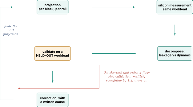
Correcting the model is where correlation either produces knowledge or produces folklore, and the difference is one step.
The right procedure is to attribute the discrepancy to a named cause, apply a correction that follows from that cause, and then validate the corrected model against a workload that was not used to derive the correction. Without the held-out check you have not built a model, you have fitted a curve to one point, and it will fail on the next workload while carrying the authority of having been "correlated to silicon."
Corrections then have to be recorded with their cause and an expiry condition, because a correction whose cause has been fixed in the next design is now an error. "Multiply the fabric's dynamic by 1.15 because the clock-tree model under-counts gater endpoints, revisit when the RTL CTS model is updated" is a maintainable artefact. "Fabric factor 1.15" written on a wiki three years ago by somebody who left is not, and every mature team has a few of those it is afraid to touch.
The failure mode to name explicitly, because interviewers like hearing it named, is the blanket fudge factor. Silicon is 20 percent high, so every number in the flow gets multiplied by 1.2. It works, in the narrow sense that the total now matches. It is also the end of learning, because the real cause is now hidden under a correction that compensates for it on average and gets it wrong per-block in exactly the pattern of section 3.3, and the next chip inherits the factor without inheriting the reason.
08.Part 8, the tool landscape, by name
These roles screen on this vocabulary, so the names have to be available instantly. Everything below is stated at the level of what class of thing each product is, sourced from public vendor material. Do not go further than this in an interview. Claiming knowledge of a tool's internals or of version-specific behaviour you have not personally used is a fast way to be caught by somebody who has, and "I know what it does, I have not driven it" is a completely respectable answer.
The organizing idea, which survives products being renamed and companies being acquired, is that there are only four jobs.
Job one, produce activity. Simulators, emulators, and the file formats of Part 4.
Job two, estimate early. RTL-stage power estimation, where no netlist exists.
Job three, check and optimize structurally. Static RTL-stage checks that find missing gating and verify power intent, plus the synthesis-side optimization that inserts gating and swaps thresholds.
Job four, sign off. Gate-level and post-layout analysis that produces the committed number, and the power-integrity analysis that consumes it.
| Product | Vendor | Class of thing |
|---|---|---|
| PrimeTime PX | Synopsys | gate-level power analysis layered on the PrimeTime timing engine. Average power from SAIF or user-specified activity, peak and time-based power from a VCD |
| PrimePower | Synopsys | the current-generation power analysis product positioned as RTL-to-signoff, supporting event-based analysis from vectors and statistical vectorless analysis, average and peak, clock and glitch power, multi-voltage |
| Power Compiler, inside Design Compiler and Fusion Compiler | Synopsys | the optimization side rather than the analysis side, covering clock gating insertion, multi-threshold cell selection, power-driven optimization, and the rtl2saif forward-annotation half of the SAIF handshake |
| PowerArtist | Ansys | RTL power analysis and reduction, with a calibration flow, publicly named PACE, that builds RTL power models from a post-layout design so RTL estimates track signoff, plus RTL-stage clock tree modelling and reduction checks |
| Joules RTL Power Solution | Cadence | RTL power with implementation-quality gate and wire estimates and time-based analysis, publicly positioned as correlating within 15 percent of Cadence's own Voltus signoff |
| SpyGlass Power family, now within the VC static platform | Synopsys, originally Atrenta | RTL-stage static analysis: power estimation, power reduction checks that report gating and activity-reduction opportunities, and power verify style structural checks on UPF intent |
| VC LP | Synopsys | static low-power verification of UPF against the design, including power state tables, shutdown, and multi-rail macros |
| PowerPro | Siemens, originally Calypto | RTL power optimization, notably sequential clock gating derived from observability and stability analysis, and emulation-driven power flows with Veloce |
| Voltus | Cadence | power integrity signoff, meaning IR drop and electromigration on the power delivery network, consuming the power numbers rather than producing them |
| RedHawk-SC | Ansys | the same class as Voltus from the other vendor |
| Palladium Dynamic Power Analysis | Cadence | emulation-driven power profiling over very long workloads |
| ZeBu Empower | Synopsys | the same, on the ZeBu emulation platform, publicly described as feeding the power-critical blocks and time windows it identifies forward into PrimePower, which is the two-phase flow of section 4.5 shipped as a product |
| Veloce Power App | Siemens | the same, on the Veloce platform, paired with PowerPro |
Two closing observations that are worth more than the table.
Analysis and reduction are different products and often different teams. PrimeTime PX and PrimePower tell you what the power is. Power Compiler and PowerPro change it. PowerArtist and the SpyGlass Power reduction checks straddle both by reporting opportunities rather than just magnitudes. When a role description says "power analysis," find out during the interview whether the role owns the measurement, the reduction, or both, because they are quite different jobs and the honest answer to "what have you done" differs between them.
Sequential clock gating deserves its own sentence because it is the one reduction technique the physics notes do not cover. Ordinary clock gating, per Part 3 of Power Fundamentals and Clock Gating, stops a register when it will not change this cycle. Sequential clock gating goes further and stops a register when its value will not be observed for some number of cycles downstream, or when it is provably stable across a multi-cycle computation, which requires reasoning across pipeline stages rather than within one. That is a genuinely different analysis, it finds savings ordinary gating cannot, and it is the reason such tools ship a sequential equivalence checker alongside, because the transformation is not combinationally equivalent and a plain LEC run per section 7.1 of Verification Methodology would fail it.
09.Part 9, where UPF sits in this flow
Part 8 of Power Fundamentals and Clock Gating already covers what UPF is, that it is IEEE 1801, what a UPF file declares, what power-aware simulation does with it, and what static power-intent checkers catch. Do not reread it here. This section covers only the part note 17 does not, which is what UPF does to the numbers.
A power model is only as good as its domain state. Consider a block in a domain the design will power down for 90 percent of a workload. An ordinary, power-unaware simulation has no notion of supply, so it simulates that block continuously, its nets toggle continuously, and the SAIF you extract charges you for switching power the silicon will never burn. The projection comes out high, someone spends a month optimizing a block that was already off, and the correlation against silicon then comes out mysteriously low.
Run the same stimulus through a power-aware simulation, which reads the UPF alongside the RTL, and the block's logic corrupts to X while unpowered, the isolation cells emit their clamp values, and the activity you extract reflects a chip that actually powers things down. That is the same SAIF file format and a materially different power number, and the difference is a file the RTL never mentions.
Three flow consequences follow, and they are the substance of this part.
The power state table is the scenario list. Section 6.1 built a budget from concurrency scenarios. Those scenarios are not free-form prose, they correspond to legal entries in the UPF power state table. A scenario the table forbids does not need budgeting. A scenario the table permits and nobody budgeted is a hole. Reading the two documents against each other is a genuinely useful review that almost nobody does.
Static low-power checks are a precondition for trusting a power number, not just for functional correctness. A missing isolation cell is famous as a functional bug. It is also a modelling bug, because it means the tool's picture of where the domain boundary lies does not match the netlist's, and boundary cells have power of their own. Run the static checks before you believe the analysis.
Retention and always-on logic are permanent leakage line items. Retention flops, per section 6.4 of Power Fundamentals and Clock Gating, keep a shadow latch alive on an always-on rail. Always-on wake logic leaks by definition. Both are small per instance and both are on all the time, so in a product that spends most of its life in a low-power state they can dominate the average. A budget that only tallies active-state power has omitted the state the device is actually in most of the time, and for a battery-powered product that is the whole ballgame.
10.Part 11, interview questions with model answers
Sixteen questions of the kind these roles actually ask, each with an answer written the way it should be spoken rather than the way a textbook would state it, the follow-up that is coming, and where the trap is.
Q1. "Walk me through how you would estimate the power of a block that has no netlist yet."
Answer. "I would start by being clear about what the estimate is for, because the answer changes. If it is to choose between two microarchitectures, I want a relative number and I do not need it to be accurate in absolute terms, I need it to rank the options the same way signoff eventually will. If it is to check a budget, I need absolute accuracy and at RTL I probably cannot get it, so I would say so rather than deliver a number I do not believe.
Mechanically, at RTL, an estimation tool synthesizes a quick internal netlist and applies activity, either from an RTL simulation or vectorlessly. The activity is where the error is, so I would annotate everything I actually know, meaning the clock, the block's interface toggle rates, memory access rates, anything a designer can state a fact about, and let the tool propagate statistically only into the interior. That collapses the biggest error term.
The one thing I would flag straight away is the clock tree, because it is roughly a third of dynamic power and it does not exist yet at RTL, so whatever the tool assumes about buffer count and wire length is carrying a third of my answer."
Follow-up. "How much would you trust that number?"
Handling it. Do not name a percentage. Say the band depends overwhelmingly on whether the RTL model has been calibrated against your own previous post-layout data, that vendors publish figures in the region of 15 percent under their own conditions, and that the honest way to establish your own band is to take a finished block, run the RTL flow on it, and compare against its signoff number. That is a concrete proposal rather than a hedge, and it is the right answer.
Q2. "Vector-based or vectorless. When do you use each?"
Answer. "They answer different questions. Vector-based gives me the exact power for the stimulus I ran, so its error is not modelling error at all, it is whether the stimulus resembles the workload. Vectorless gives me the expected power under an assumed statistical model of the inputs, propagated through the logic under an independence assumption, so it has two extra error sources, the input assumption and the correlation between signals.
In practice I would not treat them as alternatives. The useful flow is hybrid, annotate the activity you know and let the engine propagate only where you genuinely have no information. Pure vectorless is right when no vectors exist yet, when I am comparing two options where the same bias cancels, and for leakage, which barely depends on activity anyway."
Follow-up. "Give me a case where vectorless is badly wrong."
Handling it. Go straight to reconvergent fanout. An AND of a signal and its own complement is constant zero and never toggles, but an engine that multiplies signal probabilities reports 25 percent occupancy and a healthy toggle rate. That structure is everywhere, in every mux tree and every one-hot decoder. Then say that commercial engines handle correlation to a bounded depth and give up beyond it.
The trap. The question sounds like it wants you to pick a side. It does not. Picking a side is the wrong answer.
Q3. "What is in a SAIF file, and what can you not do with one?"
Answer. "Per net, a toggle count and the time spent in each state, conventionally the toggle count plus time at zero, time at one, and time unknown, plus set and reset statistics for sequential cells. It is ASCII and hierarchical, and it mirrors the design hierarchy.
What it deliberately throws away is time. It keeps how many, not when. So the file is one small record per net rather than one record per event, which means, and this is the property that matters, the file size does not grow with how long you simulated. A billion-cycle run and a thousand-cycle run produce the same size file.
What that costs you is everything time-dependent. No peak power, no power waveform, no di/dt, no answer to when in the run something happened. For that you need VCD or FSDB, which keep every event with its timestamp and are correspondingly enormous."
Follow-up. "How do you annotate a gate-level netlist from RTL activity when the names have all changed?"
Handling it. This is the forward-and-backward SAIF handshake, and it is the answer that separates flow experience from reading. The synthesis tool writes a forward SAIF from the elaborated design telling the simulator what to monitor and in what naming scheme, the simulator writes a backward SAIF with the measured counts, and the tool reads it back. You have to preserve RTL hierarchy names through synthesis or the mapping fails quietly. Then add the instinct. Always read the annotation coverage report before the power number, because unannotated nets silently fall back to defaults.
Q4. "Your RTL estimate said 80 mW. Post-layout says 130 mW. Where did the 50 mW come from?"
Answer. "I would decompose before I speculate, but the candidate list is short and I would go in this order.
First the clock tree, because it is the biggest single term and it is the term that did not exist at RTL. Real CTS usually needs more buffering than an early model assumes, and it needs more of it on a heavily clock-gated design because every gater is an endpoint that has to be balanced.
Second, glitch power. RTL simulation has no delays, so it structurally cannot see a node making three transitions on its way to the right answer. Glitch only ever adds, so it is a systematic under-estimate and it shows up the first time you run with real delays.
Third, wire capacitance, because before routing the wire load is an estimate and at advanced nodes interconnect is a large share of what switches.
Fourth, whether the activity actually changed. If the RTL number used one stimulus and the post-layout number used another, I am comparing two different questions and the 50 mW might not be a design fact at all.
The way I would actually find it is by differencing the reports per block and per component rather than looking at the totals, because the total tells you nothing about which of those four it was."
Follow-up. "Which of those would you fix?"
Handling it. None of them, in the sense the question invites. Three of the four are the estimate improving rather than the design worsening, and the correct response is to feed the correction back into the RTL model so the next estimate does not have the same gap. Only the fourth, a genuine activity difference, is a design or workload question. Saying that is the answer.
Q5. "How do you build a chip-level power budget?"
Answer. "The thing to get right first is that a chip budget is not the sum of the block maxima. If you sum maxima you get a number that is often fifty to a hundred percent over target and you conclude, wrongly, that the chip is impossible. The budget is the maximum over the legal concurrent scenarios, because software does not ask every block to peak at once, and where it could, something has to stop it.
So the procedure is to enumerate the scenarios that the product actually has to sustain, gaming, camera capture with inference, a CPU burst, video playback, idle with the screen on. For each one, write down what each block is doing and what that costs. The largest of those is your budget-relevant number.
Then there is the row where everything peaks simultaneously. Nothing in the silicon prevents it. What prevents it is a runtime power manager that refuses the concurrent grant, and that means the gap between the sum of maxima and the budget is a requirement on a control block, not a design flaw."
Follow-up. "Where does the margin go?"
Handling it. This is the good part of this question. Margin should be explicit, singular, and owned at the top, not buried inside each block's number. Hidden margin cannot be spent when a block overruns because nobody knows it is there, and it compounds if the integrator adds more on top, so a chip that is genuinely fine can be reported as over budget and a team can spend months optimizing a problem that does not exist.
The trap. Summing block maxima. It is the obvious answer and it is wrong, and the question is asked specifically to see whether you reach for it.
Q6. "A block comes in 40 percent over budget three months before tape-out. What do you do?"
Answer. "Before anything else I would establish whether the design got worse or the model got better, because a jump that size between two estimates is very often a methodology change, a newly annotated glitch term, a corrected clock-tree assumption, a different corner, a different activity source. Rerun the previous configuration alongside the new one and difference them. Optimizing against a number that moved for measurement reasons is pure waste and it happens constantly.
Assuming it is real, I would work cheapest first. Activity recovery, meaning per-instance reports sorted by power, ungated registers, un-isolated operands, memories read on cycles where the result is discarded. Then coarser gating or a domain restructure, which costs verification effort. Then microarchitecture, fewer ports or narrower datapath, which costs performance. Then spend the chip reserve, which is why the reserve needs to be visible. Then cap the operating point, which is very effective because of the V-squared term and directly costs the performance the block existed to deliver. Then change the product specification, which is not my call but which I should escalate early rather than late.
The ordering is the answer. Every one of those is available and they differ by an order of magnitude in cost."
Follow-up. "What if none of it is enough?"
Handling it. Say that the last two rungs are real options rather than failures, and that the failure mode is discovering this at week eleven of twelve. Then say what you would have done differently, which is to have had a budget-tracking cadence that would have caught a drift of that size before it became a 40 percent cliff.
Q7. "Silicon comes back 20 percent above your projection. Find out why."
Answer. "First I would check the measurement, because assuming the meter is right is how people waste a week. What is actually on that rail, what is the sense resistor tolerance, what is the regulator efficiency, is the telemetry calibrated, is the part at the temperature I think it is.
Then I would split the number, because one lump of discrepancy is not diagnosable and two are. Total rail power is leakage plus alpha-C-V-squared-f. Hold voltage fixed, hold junction temperature fixed, run the same workload, and sweep frequency. That is a straight line in f whose intercept is leakage and whose slope is the effective switched capacitance. Two points give me both.
Now the diagnosis forks. If leakage matches and dynamic is high, it is an activity or capacitance problem, and activity is far more likely, so workload mismatch first, then glitch, then the clock tree. If dynamic matches and leakage is high, it is not activity at all, it is process corner, junction temperature, the multi-Vt mix synthesis actually chose, or domains I believed were off not being off. If both are high in similar proportion, suspect something global like the actual operating voltage, which is guardbanded above nominal and enters as V-squared."
Follow-up. "What could go wrong with that sweep?"
Handling it. Two things, and volunteering them before being asked is better. The workload's per-cycle activity has to be frequency-invariant, so a memory-bound workload will not do because it stalls more at high frequency. And temperature has to be genuinely held, because if the die heats up with frequency then leakage rises with it, the curve bends upward, and a straight-line fit over-attributes to the slope and under-attributes to the intercept.
Q8. "How would you get realistic activity for a full software workload?"
Answer. "Simulation cannot do it, and the reason is arithmetic rather than effort. An event-driven simulator on a full SoC runs at roughly one to ten kilohertz of simulated clock. A workload worth profiling is a billion cycles or more. That is eleven days at the low end before you account for the slowdown from dumping activity.
Emulation runs the netlist at a megahertz or more, so a billion cycles is under twenty minutes, and every emulation vendor ships a power app on top for exactly this, Palladium Dynamic Power Analysis, ZeBu Empower, the Veloce Power App with PowerPro.
But you cannot dump full-fidelity activity for a billion cycles either, because the file would be petabytes. So the flow is two-phase. Pass one runs the whole workload with a lightweight accumulator producing a coarse power-versus-time curve, cheap enough to keep. Pass two takes the windows that curve flagged and replays just those with full activity for detailed per-instance analysis."
Follow-up. "What did that change, beyond being faster?"
Handling it. This is the answer that shows understanding rather than recognition. It changed power from something you estimate into something you profile, the way performance has been profiled for decades. And it made power a software-visible finding, so a driver polling a register at a kilohertz, or a firmware loop that never lets a domain reach the residency break-even, is now findable before tape-out and fixable in software at a thousandth of the cost.
Q9. "You have 95 percent clock gating coverage. How did you measure it, and what did it save?"
Answer. "Start with the definition, because three different things get called clock gating efficiency and they give different numbers on the same design. Flop coverage is the fraction of flops with a gater in front, and it is the weakest, because it counts a four-flop group and a sixty-four-flop group the same and says nothing about whether the enable is ever low. Clock-power-weighted coverage is better because it credits a coarse gater for its whole subtree, but it is still a static structural measure of what could be saved. Dynamic gating efficiency simulates a workload and counts the flop-clock-cycles actually suppressed, and that is the one that corresponds to power on a bench.
My number is clock-power-weighted, measured across the regression workload set, with every gater's enable coming from a real idle or update condition.
And coverage is not savings. If gated flops are 95 percent of clock power and their enables are low seventy percent of cycles on average, the saving is 0.95 times 0.70 of the clock power, so about two thirds of it. Against total block dynamic power where the clock is a third, that is roughly a twenty percent cut, not a ninety-five percent one."
Follow-up. "How did you find the ungated logic?"
Handling it. Per-instance power reports from a gate-level netlist with annotated switching activity, sorted descending by clock power and filtered to ungated instances. The list is short because power distribution is heavily skewed. Each entry closes either with an RTL rewrite that gives synthesis a provable enable, or with a written reason. Then the second, coarser pass over whole blocks looking for architectural idle windows, which is where the large wins are.
The trap. Quoting 95 percent as though it were a power saving. The interviewer is very likely to let you do it and then ask what it saved. Volunteering the distinction before being asked converts the trap into your best moment.
Q10. "What power analysis tools have you used?"
Answer. "Let me separate what I have owned from what I know. I have owned a synthesis and static timing flow end to end, which necessarily includes the power-adjacent parts of it, clock gating insertion, multi-threshold optimization, and SAIF annotation, and I drove clock gating work from per-instance power reports. What I have not personally owned is a chip-level power budgeting and silicon correlation flow.
On the landscape, I would place the products in four buckets rather than list them flat. Activity production is simulators and emulators plus SAIF, VCD and FSDB. Early estimation is PowerArtist and Joules. Structural checking and reduction is the SpyGlass Power family and PowerPro on one side and Power Compiler on the synthesis side. Signoff is PrimeTime PX and PrimePower for the power number, and Voltus or RedHawk for the power-integrity side that consumes it."
Follow-up. "Could you pick up our flow?"
Handling it. The answer is not "yes." It is to name what transfers, which is the flow-ownership discipline, the annotation and coverage habits, the corner and conditions discipline from timing closure, and the debugging instinct of decomposing a discrepancy before explaining it, and then name what you would need, which is the tool's specific commands and the team's specific calibration history.
The trap. Listing tools you have read about as though you have driven them. Anyone who has driven them will find out in one follow-up. The bucketed answer demonstrates more understanding than a list would, and it is entirely honest.
Q11. "What is the danger of a global default toggle rate?"
Answer. "The danger is that the error is systematic rather than random, and correlated with what the block does, so it does not average out and a correct chip total can be correct for two large wrong reasons.
Concretely. Take a default of 0.2 toggles per cycle applied to a 600 picofarad block at 0.8 volts and 2 gigahertz. That is 76.8 milliwatts for any block of that size, regardless of function. A video line buffer holds correlated pixel data, so its upper bits barely move, and its real weighted activity is about 0.0775 in the zero-to-one convention, giving 59.5 milliwatts. The default over-estimated by 29 percent, which is wasteful but safe. A cipher datapath produces intermediate values designed to look uniformly random, so every node sits near 0.25, giving 192 milliwatts. The default under-estimated by a factor of two and a half.
Now put seven video-class blocks and one cipher block on a chip. The default total is 614 milliwatts, the real total is 609. Under one percent error at chip level. And the cipher block is at two and a half times its budget, so its local grid is undersized, it is a thermal hotspot the floorplan did not anticipate, and its switch-in di/dt is two and a half times what the droop analysis assumed."
Follow-up. "So what do you do about it?"
Handling it. Annotate rather than default wherever a fact is available, treat blocks whose data statistics are known to be unusual as requiring annotation rather than defaults, and above all check the budget per block and not only at the top. A methodology that only validates the total is not validating anything.
Q12. "How does UPF affect the power numbers, not just the functionality?"
Answer. "Most obviously through the activity. An ordinary simulation has no notion of supply, so a block your design will power down for ninety percent of a workload gets simulated running for a hundred percent of it, and the SAIF you extract charges you for switching the silicon never does. Power-aware simulation reads the UPF alongside the RTL, corrupts unpowered logic to X, models the isolation clamps, and models retention, so the activity you extract reflects a chip that actually powers things down. Same file format, materially different number.
Second, the power state table is effectively the scenario list you budget against. A concurrency the table forbids does not need a budget, and one it permits that nobody budgeted is a hole. Reading the budget scenarios against the power state table is a review almost nobody does.
Third, retention and always-on logic are permanent leakage line items. Small per instance, on all the time, and in a product that spends most of its life in a low-power state they can dominate the average."
Follow-up. "Have you written UPF?"
Handling it. Answer honestly. If the power architecture in your flow was captured elsewhere and you worked on the logic it drove, say exactly that, then demonstrate you know what belongs in the file, meaning supply nets, domains, switches, power states, isolation strategies, level shifter strategies, retention strategies. Knowing the contents and being straight about not having authored the file is a perfectly strong position. Implying otherwise fails the next question.
Q13. "How do you compare two microarchitectural options for power before either exists?"
Answer. "The metric has to be energy per operation rather than power, per section 1.4 of DVFS Droop and Thermal, because power alone rewards being slow. If option A burns less power but takes twice as many cycles, it lost.
Then the key insight is that I do not need absolute accuracy, I need the ranking to be right. Both estimates carry the same systematic bias from the same uncalibrated model, and in a ratio most of that bias cancels. So I would build both at a level of detail that is comparable, hold everything else identical, meaning same activity assumptions, same technology assumptions, same clock tree model, and compare.
What I would watch for is any difference between the options that the shared model handles asymmetrically. If option A is register-heavy and option B is memory-heavy, and my model is well calibrated for logic and poorly for memory, then the bias does not cancel and the ranking is not safe. That is the thing to look for before trusting a comparison."
Follow-up. "How big does the difference need to be before you believe it?"
Handling it. Say honestly that this is a judgment call, that a 2x difference at RTL is almost certainly real and a 5 percent one almost certainly is not, and that the way to establish your own threshold is to look back at previous projects where an RTL comparison was later checked against signoff. That is a hedged answer, and it is the correct one, because inventing a threshold is worse.
Q14. "Why do you care about peak power separately from average?"
Answer. "They constrain completely different things and neither substitutes for the other.
Average power over a long window sets thermal behaviour and battery life, because thermal mass smooths over microseconds. Peak power over a short window sets what the power delivery network has to supply, and it matters through di/dt rather than through heat, because a large current step through the package inductance produces a voltage droop, and if that droop takes the rail below the minimum operating voltage the chip fails timing.
Which means peak power analysis needs a completely different activity file. An averaged SAIF has no time information at all, so it cannot produce a peak, no matter how good the tool is. You need a VCD or FSDB and a time-based analysis."
Follow-up. "What is the right window for peak?"
Handling it. Say that it depends on the resonance being protected against, that the power delivery network has multiple droop mechanisms operating on different timescales from roughly a nanosecond to microseconds, and that the answer therefore comes from the power integrity team's model rather than from a rule of thumb. Naming that the window is set by the physics of the PDN rather than by convention is the point. Then defer, and say that the mitigations, decoupling capacitance, staged wake, adaptive clocking, and droop detection, are the other half of the answer.
The trap. Treating peak power as "the highest average I measured." A peak that is defined over a millisecond window is an average, and it will not catch anything.
Q15. "How do you know your power model is right?"
Answer. "You do not, until you have compared it against something you did not use to build it. That is the whole discipline.
Correlation is a loop. You project, you measure, you decompose the discrepancy into leakage and dynamic, you attribute it to a named cause, and then, crucially, you validate the corrected model against a held-out workload. Skipping the last step means you have fitted a curve to one point and it carries the authority of having been correlated to silicon, which is worse than having no correction at all.
Corrections have to be recorded with their cause and an expiry condition, because a correction whose cause has been fixed in the next design is now an error."
Follow-up. "What is the failure mode you have seen?"
Handling it. The blanket fudge factor. Silicon is 20 percent high so everything gets multiplied by 1.2. It makes the total match, and it ends the learning, because the real cause is now hidden and the correction is wrong per-block in exactly the pattern of the toggle-rate example. The next chip inherits the factor without the reason. If you have not personally seen this, say so and say you would expect it, which is an honest framing of a known failure mode.
Q16. "Design a power analysis flow for a new block, from scratch."
Answer. "I would build it in the order the information becomes available, and I would define at each stage what decision the numbers support, because that is more useful than chasing accuracy.
At RTL, before anything is synthesized, I want two things. A relative comparison capability for architecture choices, and a structural report, meaning ungated registers, un-isolated operands, speculative memory reads. Those findings do not depend on the activity assumption being right, so they are trustworthy at a stage where the magnitudes are not.
At synthesis, I want the annotation handshake working end to end, forward SAIF out, backward SAIF in, and I want to check annotation coverage as a flow gate. An unannotated flow silently degrades to vectorless with defaults and nobody notices.
At gate level with delays, I want glitch power to appear for the first time, and I want per-instance reports sorted by power as the work queue.
At post-layout, I want the committed number with real parasitics and a real clock tree, at a stated operating point, with the conditions vector written at the top of the sheet.
Alongside all of that, I want activity from emulation as early as I can get it, because the single largest error term is workload representativeness and no amount of tool accuracy fixes it.
And I want a correlation plan written before silicon exists, meaning which rails are instrumented, which workloads will be run, and how the leakage-versus-dynamic decomposition will be done. Writing that after the parts arrive is how a month gets lost."
Follow-up. "What would you do first if you joined and none of that existed?"
Handling it. Build the measurement before building the optimization. Get one block's RTL estimate compared against its own post-layout number so the team has an empirical error band instead of a vendor's, and get annotation coverage reported as a gate. Those two are cheap, they take weeks not quarters, and everything downstream is untrustworthy without them. Then say the thing that makes it credible. This is the same instinct as the clock gating work, where the useful contribution was building the per-instance measurement first and the RTL edits were the easy part afterwards.
11.Part 13, check yourself
Answer out loud, in full sentences, as if an interviewer asked. If you cannot, reread the section named.
- Compute the power of an 8-bit register from a twenty-cycle value trace by hand. What are the only two ingredients any power tool needs, and which of the two is hard? (1.1, 1.2)
- Why is a power number without a stated window, workload, voltage, frequency, temperature, and corner not yet a fact? Give three different numbers derivable from one power trace. (1.4)
- A signal is quoted as having a toggle rate of 0.3. What must you ask before using it, and what does getting it wrong cost you? (2.2)
- Vector-driven analysis is exact given the stimulus. So where does its error come from? Name the main term and three secondary ones. (2.4)
- Draw the two-gate circuit where vectorless probability propagation gets the answer completely wrong, and say what the structure is called and why it is common. (3.1)
- Work the toggle-rate default example, with two blocks, one over-estimated and one under-estimated, and a chip total that comes out right. What is wrong even though the total is right? (3.3)
- Give three situations where vectorless is the right tool despite everything in question 5. (3.4)
- Size a VCD for 100,000 nets over a million cycles. Now size the SAIF. What property of the SAIF size is the important one? (4.1, 4.2)
- Explain the forward and backward SAIF handshake and what it is solving. What report do you read before you read the power number? (4.2)
- Why can simulation never produce activity for a real software workload? Do the arithmetic. What replaced it, and why is the emulation power flow necessarily two-phase? (4.4, 4.5)
- Name the four estimation stages and say what decision each can support. Why is the largest single term in the budget also the least knowable early? (5.1, 5.2, 5.3)
- Six blocks sum to 8.5 W against a 5.0 W target. Explain why the chip is nevertheless feasible, and what has to exist for it to be feasible. (6.1)
- Why is hidden margin worse than no margin, and how does it compound? (6.2)
- Block A and block B each report 0.40 W. Why might their sum be nearer 1.8 W than 0.8 W? Do the voltage and temperature arithmetic, then say what is wrong with applying a doubling rule to one variable at a time. (6.3)
- Give the escalation ladder for a block that comes in over budget, in cost order, and say what step zero is and why people skip it. (6.4)
- Silicon is 20 percent above projection. Describe the frequency sweep that splits the discrepancy into two, work the arithmetic on two measured points, and give both caveats. (7.2)
- List the common discrepancy sources between projection and silicon, and give the direction each one pushes. (7.3)
- What is the one step that separates a correlated model from a curve fitted to a single point? What is the blanket fudge factor and why is it a failure? (7.4)
- Place PrimePower, PowerArtist, Joules, the SpyGlass Power family, Power Compiler, and Voltus into the four job buckets. What is sequential clock gating and why does it need a sequential equivalence checker? (8)
- How does UPF change a power number rather than just a function? Give the activity argument, the scenario argument, and the always-on argument. (9)
- Convert "I got 95 percent clock gating coverage" into a methodology claim, and convert "I built a resource controller IP" into a budget-enforcement claim. (10.1, 10.2)
12.Part 14, related notes
- Power Fundamentals and Clock Gating for the physics this note assumes throughout, meaning , the activity factor, leakage and its temperature dependence, clock gating and the three definitions of its efficiency, power domains, the power-down and power-up sequences, and UPF as a language rather than as a flow input
- DVFS Droop and Thermal for what consumes the peak-power numbers this note explains how to produce, meaning droop, , the power delivery network, guardband, and adaptive clocking, and separately section 1.4 there for why energy per operation rather than power is the right metric when comparing two options, which Q13 in Part 11 leans on
- Verification Methodology for simulation speed in 8.1, which sets the ceiling in Part 4 here, for emulation and FPGA prototyping in 8.2, for gate-level simulation in 8.3, and for the formal material that Part 9's power-intent checking sits alongside
- STA Synthesis and Physical Design for the implementation flow this power flow rides alongside, for parasitic extraction, for corners and derating, and for the conditions discipline that section 6.3 depends on
- Reliability Aging and Variation for process variation and part-to-part spread, which is one of the named silicon-correlation discrepancy sources in 7.3
- SRAM Arrays and ECC for memory arrays, whose vendor power models are a frequent and frequently under-examined term in a block budget
- Performance Modeling Part 7 for the correlation discipline on the performance side, which is the same loop as Part 7 here applied to a different quantity, including the held-out-validation habit and the discrepancy-attribution categories
- DFT and Silicon Debug for the post-silicon side generally, and for why what is on which rail is partly a debug-observability decision
- RTL Design and SystemVerilog for the coding patterns that let synthesis prove an enable, which is what makes a gating opportunity closable
- Apple Context and Behavioral for how to frame the resume conversion in Part 10 inside a behavioral loop
- From Logic to Silicon for the vault's circuit-level treatment of CMOS switching power
- Power, Frequency, and Thermal for the vault's architectural treatment of frequency, thermal limits, and dark silicon