Branch Prediction Foundations
September 13, 202622 min readadvanced
The five-stage pipeline of Chapter 29 suffered a two-cycle bubble on every taken branch because the front end did not know the branch outcome until the execute stage. The deeper pipelines of Chapter 30 made…
The five-stage pipeline of Chapter 29 suffered a two-cycle bubble on every taken branch because the front end did not know the branch outcome until the execute stage. The deeper pipelines of Chapter 30 made the cost worse, because a 15-stage pipeline pays 15 cycles per misfetch instead of 2. Modern out-of-order cores have front-end depths of 10 to 20 cycles, so an unpredicted branch costs roughly half the IPC of a useful instruction. With one branch in every five instructions on typical code, a core that fetched serially would lose 80 percent of its potential throughput to branch stalls.
Branch prediction breaks this dependence chain by guessing each branch’s outcome at the fetch stage, before the branch has even been decoded. The front end keeps fetching on the predicted path. By the time the branch resolves in the back end, the predicted path has accumulated dozens of in-flight instructions. If the prediction was right, those instructions are useful. If the prediction was wrong, the core flushes them and refetches. Modern predictors are right between 96 and 99 percent of the time on typical code, so the bet pays off heavily on average.
This chapter develops branch prediction from first principles. It starts with the cost of a misprediction in a deep pipeline, develops the bimodal one-bit and two-bit direction predictors, adds history correlation through the global history register and the gshare and gselect schemes, treats the agree predictor, and covers target prediction through the BTB and indirect target predictor. The chapter closes with the return address stack and the role of confidence estimation. The modern tagged-history predictors (TAGE, ITTAGE, BATAGE) and the perceptron family are the subject of Chapter 56.
01.The Cost of a Misprediction
A modern x86-64 core has a front end depth of 10 to 14 cycles from the PC generator to the renamer. The back end adds another 5 to 10 cycles before the branch resolves in execute. A branch misprediction discovered at execute therefore costs at least 15 cycles of recovery, sometimes 25 cycles, plus the cycles spent issuing the wrong-path instructions through the back end before the misprediction was detected.
A concrete numerical example sets the stakes. Assume the core fetches 6 instructions per cycle and executes 4 instructions per cycle. A branch misprediction discovered after 20 cycles wastes roughly instruction slots in the back end. If 20 percent of executed instructions are branches and the predictor is right 96 percent of the time, the per-branch wasted-slot contribution is wasted slots per executed instruction. Each useful instruction then costs issue slots instead of one, so the actual IPC ceiling is about instructions per cycle, a 39 percent loss to mispredictions alone.
If the predictor accuracy drops to 90 percent, the loss grows to wasted slots per executed instruction, which collapses the achievable IPC to roughly . This is why each percentage point of misprediction-rate improvement matters. On a wide deep machine, the cost of mispredictions dominates almost every other performance lever.
The recovery depth depends on where the misprediction is detected. If the front end has a fast resolution path (the branch is conditional on a register that was computed early), the misprediction can be caught at decode and the recovery is short. If the branch resolves in the back end (the conditional operand depends on a long-latency operation), the recovery can be 20 to 30 cycles. Some designs implement a checkpoint mechanism that snapshots renamer state at branches and rolls back without flushing the front-end pipeline, which reduces the recovery cost at the price of checkpoint storage. The fundamentals do not change: a misprediction costs cycles, and the cost grows with pipeline depth.
02.One-Bit and Two-Bit Direction Predictors
The simplest direction predictor remembers, for each branch, the last outcome of that branch. A 1-bit prediction table indexed by the low-order bits of the branch PC records "0" for not-taken and "1" for taken. On a fetch, the predictor reads the table at the branch’s PC index and predicts the recorded value. After the branch resolves, the table is updated with the actual outcome.
This 1-bit scheme captures the locality that most branches behave the same way most of the time. Loop back-edges are taken almost always until the loop exits. Forward branches in error-handling code are almost never taken. A 1-bit predictor is right whenever the branch’s behavior is unchanged from its last execution, which is most of the time.
The weakness of the 1-bit predictor is the loop-exit pattern. A loop that iterates 100 times takes the back-edge 99 times and falls through once. A 1-bit predictor mispredicts twice per loop: once on the fall-through (the last iteration), and once on the re-entry into the loop the next time around. The second misprediction is the expensive one. After the loop exits, the predictor remembers "not-taken" for that branch. When the loop is re-entered (a higher-level loop iterates), the predictor’s first prediction is wrong.
The two-bit saturating counter, introduced in Smith’s 1981 paper [1], solves the loop-exit weakness. The counter has four states. State 00 strongly predicts not-taken, 01 weakly predicts not-taken, 10 weakly predicts taken, and 11 strongly predicts taken. A taken outcome increments the counter (saturating at 11), and a not-taken outcome decrements it (saturating at 00). The two-bit FSM is shown in Figure 1 below.
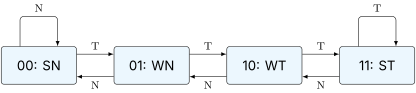
The improvement comes from the hysteresis. A single contrary outcome moves the counter from strong to weak but does not flip the prediction. The loop back-edge sits in state 11 (strong taken) across the loop’s lifetime. The exit moves it to 10 (weak taken). The re-entry, which is taken, moves it back to 11. The 1-bit predictor’s second misprediction is gone.
The two-bit predictor with a table of entries indexed by the low-order bits of the branch PC is called the bimodal predictor. The naming captures that the predictor recognizes two modes per branch: taken and not-taken, each with a confidence level. The bimodal predictor’s storage cost is bits. A 4 KiB bimodal PHT holds 16384 two-bit counters and gives accuracy in the 88 to 92 percent range on typical code, depending on the workload.
03.Correlation and Global History
A bimodal predictor is right most of the time, but it cannot catch correlated branches. Consider the code pattern:
Correlated branches that the bimodal predictor cannot separate
| if (x == 0) { ... } // branch A | |
| if (y == 0) { ... } // branch B | |
| if (x == 0 && y == 0) { ... } // branch C |
Branch C is taken only when branches A and B were both taken. A bimodal predictor sees branch C in isolation. It can learn the fraction of executions that take C, but it cannot learn the correlation: that C is taken whenever the previous two branches were taken. To capture this, the predictor needs to remember the recent history of all branches, not just the branch’s own history.
The global history register (GHR) is a shift register that records the outcome of the most recently executed branches. The GHR holds a single bit per branch, with 1 for taken and 0 for not-taken. After each branch resolves (or, in some designs, after each branch is predicted), the outcome is shifted into the GHR’s low bit, and the high bit is discarded. A GHR of length 14 to 20 bits is typical in modern designs.
The PHT index then combines the branch PC and the GHR. Different combination schemes give different predictor flavors, each trading off in subtle ways.
The Two-Level Predictor and gselect
Yeh and Patt’s two-level adaptive predictor of 1991 was the first to formally exploit global history [2]. The simplest two-level scheme, gselect, concatenates the low-order bits of the branch PC with the GHR. If the GHR is bits and the PC takes bits, the PHT is entries of two-bit counters. Each combination of PC bits and history bits has its own counter, so the predictor can distinguish "branch C with history 11" from "branch C with history 00" and learn that the first is taken and the second is not.
The cost of gselect is the table size. For and , the PHT is bits = 256 KiB, which is large. Most PCs only use a few of their bits productively, so concatenation wastes table entries that never get accessed.
gshare
McFarling’s 1993 paper introduced gshare, which XORs the GHR with the PC bits instead of concatenating them [3]. The PHT index is therefore , where the GHR is padded or truncated to match the PC bit width. The PHT size is now entries instead of .
The XOR mixing has a subtle benefit. Multiple PC values combined with multiple histories can land in the same PHT entry, but the collisions are spread evenly across the table because the XOR is a hash. Two different PC-history combinations that have very different counter values usually do not collide, because their XOR signatures differ. At the same table size gshare is therefore more accurate than gselect, because the XOR folds all bits of context into the index while concatenation has to truncate the history and the PC to fit, and it reaches that accuracy with a -entry table instead of a -entry one.
The Agree Predictor
The agree predictor is an optimization that further reduces storage cost. Instead of storing the actual prediction in the PHT, it stores whether the predictor agrees with a static prediction stored elsewhere (typically the branch’s bias bit, set at decode based on the branch direction hint). The PHT counter is incremented when the actual outcome matches the static prediction and decremented otherwise. The predictor reads the counter and the static prediction, and outputs "agree" or "disagree."
The benefit is that branches with strong bias agree with the static prediction in nearly every execution, so the PHT counter saturates at "agree" and the prediction is correct without exercising the table’s storage capacity. The PHT entries for strongly biased branches all sit at the same saturated value, which tolerates aliasing well. A collision between two strongly- biased branches both predicts "agree" and both are right.
04.Target Prediction
Direction prediction tells the front end whether to take a branch. Target prediction tells it where to fetch from if it does take. The two predictors are separate because the answers come from different places. The direction prediction is a single bit. The target is a 64-bit address, or some compressed form of one.
Most branches are direct branches. The target is encoded as an immediate offset in the instruction. On RISC-V, beq and bne have a 12-bit signed offset, giving a range of KiB. The jal instruction has a 20-bit offset, giving MiB. j, the alias for jal x0, label, has the same range. AArch64’s b.cond has a 19-bit offset, and the unconditional b has a 26-bit offset. On x86-64, branches have 8-bit, 16-bit, or 32-bit displacement forms.
For a direct branch, the target is fixed at compile time. Once the instruction is decoded, the target is just the PC plus the offset, which is simple integer arithmetic. The challenge is that the front end must predict the target before decode, at the fetch stage. The instruction has not been parsed yet. The front end does not know whether the byte at PC is a branch at all, let alone what its offset field is.
The Branch Target Buffer
The branch target buffer (BTB) solves this. It is a cache, indexed by branch PC, that records the most recent target address for that PC. On a fetch, the BTB is consulted in parallel with the I-cache. If the BTB has an entry for the current PC, two things happen: the front end learns that the byte at PC is a branch (the implicit fact of a BTB hit), and it learns the target. The next fetch can issue from the target on the next cycle, with no decode-delay bubble.
A typical BTB is sized at 4 K to 16 K entries on modern x86-64 cores. The entries are tagged so that two different PCs cannot collide silently. Each entry holds the target address (or a compressed delta from the branch PC), the branch type (direct, indirect, return, call), and sometimes a small confidence counter. The total storage is a few tens of kilobytes.
The BTB miss case is the slow path. If the branch is not in the BTB, the front end does not know it is a branch and proceeds with sequential fetch. The branch is detected at decode (one to three cycles later), at which point the target is computed and a refetch is issued. The bubble is 1 to 3 cycles, which is much less than a full misprediction recovery but still measurable.
Table 1. Direct branch target prediction options
| Prediction source | Cycle available | Cost on hit |
|---|---|---|
| BTB (no decode needed) | 1 cycle | 0 bubble |
| Decode (offset from instr) | 3 cycles | 2 bubbles |
| Execute (recomputed) | 16 cycles | 15 bubbles |
Source: synthesized from Intel and AMD optimization guides. Numbers approximate for a 5 GHz core.
Indirect Branch Targets
The harder problem is indirect branches. An indirect branch’s target is computed from a register or memory operand at run time, not encoded in the instruction. Examples include virtual function dispatch in C++, switch statements compiled as jump tables, function pointers in C, returns from functions (which are a special case, treated separately), and the trampolines used by dynamic linkers.
The BTB alone is not enough for indirect branches. The BTB stores one target per branch PC, but an indirect branch’s target varies across executions. A single virtual call site can dispatch to a dozen different functions in the same program run, depending on the object’s runtime type. A BTB entry that records only the last target will be right about as often as one polymorphic site favors a single class, which is often (most polymorphism is near-monomorphic at runtime) but not always.
The indirect target predictor addresses this with a separate structure that combines the branch PC with the global history (analogous to gshare for direction prediction) to index a target cache. Different histories lead to different target predictions for the same branch PC. Kalamatianos and Kaeli proposed an early version using path history [5]. ITTAGE (covered in Chapter 56) is the modern instantiation.
05.The Return Address Stack
Returns from function calls are a special case of indirect branches with a structural pattern: a return matches a prior call. The target of ret on x86-64 (or jr ra on RISC-V, or ret on AArch64) is the address pushed by the matching call instruction. The match is governed by the stack discipline of the calling convention, which is a strong hint the hardware can exploit.
The return address stack (RAS) is a small hardware stack that mirrors the software call stack. When the front end encounters a call, it pushes the return address (the address of the instruction after the call) onto the RAS. When the front end encounters a ret, it pops the RAS and predicts the popped address as the return target.
A typical RAS has 16 to 32 entries. The depth limit matters only for deeply recursive code. Most programs have call depths under 20, so a 24-entry RAS catches nearly all returns. If the program exceeds the RAS depth (deep recursion or a long chain of nested calls), the RAS wraps around and overwrites its own oldest entries. The innermost returns still pop the addresses their calls pushed, but the outermost returns find their entries overwritten and fall back to the BTB.
The RAS is one of the most accurate predictors in the front end. On well-behaved code its accuracy is over 99.5 percent. The remaining mispredictions come from setjmp/longjmp, exceptions that unwind the stack, and assembly code that does not follow the calling convention.
06.Confidence Estimation
Some predictions are stronger than others. A two-bit counter at state 11 (strong taken) is more reliable than one at state 10 (weak taken). Designs can exploit this by attaching a confidence estimate to each prediction and using the estimate to gate downstream speculation.
A simple confidence scheme reads the saturation state of the counter. State 11 or 00 is high-confidence, state 10 or 01 is low-confidence. More refined schemes maintain a separate confidence counter per branch, incremented on a correct prediction and decremented (or reset) on a misprediction. A saturating confidence counter of three bits gives finer granularity than the two-bit prediction counter.
Confidence has at least three uses in a modern core. First, it can gate speculative loads: a low-confidence branch should not issue loads down its predicted path that could cause cache or TLB fill side effects. Second, it can gate runahead execution: a low- confidence branch is a poor candidate to use as the basis for prefetching. Third, it can throttle the predictor itself: the predictor can fall back to a static prediction (perhaps the backward-taken-forward-not-taken heuristic) for branches with persistently low confidence.
07.Putting It Together: A Hybrid Predictor
Real front ends combine multiple predictors with a meta-predictor that chooses between them at fetch time. McFarling’s 1993 paper described the combination of a bimodal local predictor and a gshare global predictor, with a 2-bit selector PHT learning which of the two to trust for each branch [3]. The Alpha 21264 shipped a predictor built on this combining principle, with measurable accuracy gains over either component alone [4].
The meta-predictor’s job is to learn which branches are better predicted by local history (a branch’s own past behavior) versus global history (recent behavior of all branches). Loop branches typically prefer local history. Correlated if-then-else branches prefer global history. The meta-predictor’s counter learns this per branch.
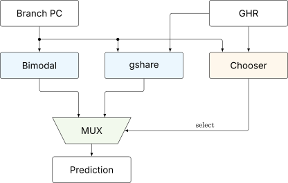
A modern front end’s predictor is more complex than this picture suggests. It typically includes the bimodal, gshare or a tagged equivalent, an indirect predictor, an RAS, a loop predictor, and a hybrid chooser. Chapter 56 develops the tagged-history predictors (TAGE, BATAGE) and perceptron predictors that have displaced gshare as the high-end direction predictor of choice in current designs.
08.Worked Examples
09.Exercises
References
- [1]Smith, James E. (1981). “A Study of Branch Prediction Strategies.” Proceedings of the 8th Annual Symposium on Computer Architecture (ISCA), pp. 135--148.
- [2]Yeh, Tse-Yu and Patt, Yale N. (1991). “Two-Level Adaptive Training Branch Prediction.” In Proceedings of the 24th Annual International Symposium on Microarchitecture (MICRO), pp. 51--61. doi:10.1145/123465.123475
- [3]McFarling, Scott (1993). “Combining Branch Predictors.” In WRL Technical Note TN-36, Digital Equipment Corporation.
- [4]Kessler, R. E. (1999). “The Alpha 21264 Microprocessor.” In IEEE Micro, Vol. 19, No. 2, pp. 24--36. doi:10.1109/40.755465
- [5]Kalamatianos, John and Kaeli, David R. (1998). “Predicting Indirect Branches via Data Compression.” In Proceedings of the 31st Annual International Symposium on Microarchitecture (MICRO), pp. 272--281. doi:10.1109/MICRO.1998.742787